library(CoseRo)
library(ggplot2)
library(dplyr)
library(tidyr)
library(sf) # for spatial outputs in Part 8
library(patchwork) # for multi-panel parameter maps
# ── Paths ──────────────────────────────────────────────────────────────────
project_path <- "C:/COSERO/MyCatchment" # adjust to your project
par_file <- file.path(project_path, "input", "para_ini.txt")
# ── Subbasins ───────────────────────────────────────────────────────────────
subbasins <- c("001", "002", "003") # adjust to your catchment
target_subbasin <- "003" # most downstream subbasin
# ── Calibration / validation periods ───────────────────────────────────────
cal_start <- as.Date("2004-01-01") # run start incl. 1-year spin-up; metrics from 2005
cal_end <- as.Date("2024-12-31")
val_start <- as.Date("1991-01-01") # run start incl. 1-year spin-up; metrics from 1992
val_end <- as.Date("2004-12-31")
# ── Plot output directory ───────────────────────────────────────────────────
plot_dir <- file.path(project_path, "module4_results")
dir.create(plot_dir, showWarnings = FALSE, recursive = TRUE)Mathew Herrnegger · mathew.herrnegger@boku.ac.at
Institute of Hydrology and Water Management (HyWa) BOKU University Vienna, Austria
LAWI301236 · Distributed Hydrological Modeling with COSERO
![]()
Introduction
Module 3 gave you a systematic picture of which parameters control your model’s behaviour and how much uncertainty remains in the outputs. This module completes the modelling cycle. You will use those sensitivity results to set up an automatic calibration, assess whether the optimised parameters generalise to an independent period, and then dissect the model’s performance from every relevant angle — hydrographs, residuals, seasonal dynamics, water balance, and spatial patterns.
Calibration is important, but not everything and not an end. Yes, the goal is to maximise a score but at the same time to understand how well your model represents the real catchment — and where it inevitably falls short. Every section in this module is designed to help you ask better questions of your model, not just produce better-looking numbers.
The CoseRo package provides all the functions needed for this workflow, from optimisation to output reading and plotting.
Part 1: Calibration & Validation — Concepts
NoteWhat you’ll learn
Understand what model calibration and validation mean, how to design a split-sample test, and what calibration fundamentally cannot fix — before writing a single line of optimisation code.
What is Model Calibration?
Model calibration is the process of adjusting model parameters so that simulated outputs match observed data as closely as possible , measured by an objective function (e.g. NSE or KGE). In a conceptual rainfall-runoff model, parameters such as soil water storage capacity, recession constants, and snowmelt thresholds cannot be measured directly at the catchment scale. Calibration is therefore an inverse problem: we infer parameter values from the response of the system rather than measuring them in the field.
The challenge is dimensionality, as we saw in the parameter estimation problem introduced in Module 2. Even with 10–15 free parameters and continuous bounds, the parameter space is effectively infinite. Spatially distributed models must specify parameter values at every zone or grid cell — if a model has 10 parameters and 10,000 grid cells, there are 100,000 unknowns to determine from a comparatively small number of discharge observations. This is a severely underdetermined and ill-posed problem (Gupta, 2026).
Manual tuning by trial and error — adjusting one parameter at a time while watching the hydrograph — is tedious and it is unlikely to find the best region of parameter space, at least measured by an objective function. Automatic optimisation algorithms search this space far more systematically. At the same time, manual tuning (“eyeball verification”) can help you understand a lot about the hydrological system you are modelling.
What is Validation?
Validation tests whether the calibrated parameter set generalises beyond the data the optimiser saw. The standard approach is the split-sample test (Klemeš, 1986): you divide your data record into two non-overlapping periods, calibrate on one, and evaluate on the other without touching any parameters.
This matters because an optimiser is, by design, very good at fitting whatever data you give it. Without an independent test, you cannot tell the difference between a model that has captured real catchment behaviour and one that has simply memorised the noise of a particular period.
Split-Sample Design
The split should ensure both periods cover a representative range of hydrological conditions. Don´t forget to configure the spin-up duration - in the COSERO run call, this is set by the argument SPINUP, e.g. SPINUP = 365.
For the Wildalpen demonstration case (data: 1991–2024), we will use:
| Period | Start | End | Length | Purpose |
|---|---|---|---|---|
| Validation | 1991-01-01 | 2004-12-31 | 14 years | Independent evaluation |
| Calibration | 2005-01-01 | 2024-12-31 | 20 years | Parameter estimation |
This is a differential split-sample test (Klemeš, 1986): calibration on the recent period, validation on the earlier one. It tests whether parameters representative of current conditions also reproduce the historical hydrology — a relevant question in catchments with detectable climate trends (e.g. glacier retreat, reduced snow fraction, changes in vegetation).
Equifinality and the Limits of Calibration
Even a well-designed calibration exercise has fundamental limitations. Because many different parameter combinations can produce similarly good hydrograph fits, a high NSE does not uniquely identify the correct parameters — this is equifinality (Beven, 2001). The problem is not a software bug; it reflects the fundamental under-determination of catchment models. As Kirchner (2006) noted, it is entirely possible to get the right answers for the wrong reasons.
More concretely, calibration adjusts parameters within a fixed model structure. It cannot compensate for:
- Wrong input data — systematic precipitation undercatch in alpine gauges will cause the calibration to suppress evapotranspiration, producing a plausible \(Q_{sim}\) but a wrong water balance. In Karst areas, a missmatch between orographic and hydrological catchment boundaries will lead to mass balance errors.
- Missing processes — a catchment with significant karst drainage cannot be well-represented by a model that assumes all subsurface flow follows a linear reservoir.
- Scale mismatches — zone-level effective parameters are not the same as point-scale physical measurements. A calibrated soil storage capacity reflects the aggregate behaviour of heterogeneous soils across a km²-scale zone.
Keep this in mind throughout: use performance metrics as diagnostics, not as proof that your model is correct.
Part 2: Setup — Libraries, Paths & Parameter Bounds
NoteWhat you’ll learn
Set up your working environment, define your calibration periods, and prepare parameter bounds — starting from the full Module 3 sensitivity set and then narrowing it down based on your results.
ImportantMake a safety copy of your parameter file first
Before running any calibration, copy your initial parameter file to a backup. The CoseRo optimisation functions work on a temporary working copy and do not modify the original, but having a backup is good practice that protects against accidental overwrites during manual operations.
file.copy(
  from      = "C:/COSERO/MyCatchment/input/para_ini.txt",
  to        = "C:/COSERO/MyCatchment/input/para_ini_backup.txt",
  overwrite = FALSE   # do not overwrite an existing backup
)
Libraries and Project Settings
Starting from Module 3 — All Sensitivity Parameters
Carry over the full parameter set from Module 3 as your starting candidate list. This is intentional: it is better to start inclusive and remove insensitive parameters than to miss an important one by starting too narrow.
# Full set from Module 3 Sobol analysis — same order, same grouping
param_names_all <- c(
  "CTMAX", "CTMIN", "RAINTRT", "SNOWTRT", "NVAR",  # snow processes
  "M", "BETA", "KBF",                               # soil + runoff generation
  "TAB1",  "TAB2",  "TAB3",                         # surface / interflow / baseflow recession
  "TVS1",  "TVS2",                                  # threshold volumes
  "PCOR",  "TCOR"                                   # input corrections
)

# Load bounds for all candidates and inspect the table
par_bounds_all <- load_parameter_bounds(parameters = param_names_all)
print(par_bounds_all[, c("parameter", "min", "default", "max",
                          "modification_type", "category")])
Review the min and max columns carefully. The default bounds in parameter_bounds.csv are designed to be conservative and physically plausible for Austrian catchments in general — but your specific catchment may justify tighter or wider ranges for individual parameters.
Narrowing Bounds Based on Module 3 Results
Use the Sobol total-effect indices (ST) and behavioural parameter ranges from Module 3 to make two decisions: which parameters to exclude and whether to tighten the bounds on any retained parameter. Here, we use parameters and tighten bounds for the Wildalpen case study. Adopt this for your catchment.
# ── Step 1: Remove parameters with negligible total-effect index ─────────────
# Parameters with ST < 0.05 across all subbasins contribute very little.
# Example: NVAR, RAINTRT, SNOWTRT, TVS2, TCOR removed as insensitive here.
param_names_cal <- c(
  "CTMAX", "CTMIN",   # snow (NVAR + RAINTRT + SNOWTRT removed — insensitive)
  "M", "BETA", "KBF",
  "TAB1", "TAB2", "TAB3",
  "TVS1",                                  # TVS2 removed — insensitive
  "PCOR"                                   # TCOR removed — insensitive
)

par_bounds <- load_parameter_bounds(parameters = param_names_cal)

# ── Step 2: Tighten bounds based on behavioural ranges from Sobol analysis ──
par_bounds$min[par_bounds$parameter == "CTMAX"] <- 5;     par_bounds$max[par_bounds$parameter == "CTMAX"] <- 8
par_bounds$min[par_bounds$parameter == "CTMIN"] <- 2;     par_bounds$max[par_bounds$parameter == "CTMIN"] <- 4.5
par_bounds$min[par_bounds$parameter == "M"]     <- 50;    par_bounds$max[par_bounds$parameter == "M"]     <- 300
par_bounds$min[par_bounds$parameter == "BETA"]  <- 0.01;  par_bounds$max[par_bounds$parameter == "BETA"]  <- 5
par_bounds$min[par_bounds$parameter == "KBF"]   <- 6500;  par_bounds$max[par_bounds$parameter == "KBF"]   <- 9000
par_bounds$min[par_bounds$parameter == "TAB1"]  <- 30;    par_bounds$max[par_bounds$parameter == "TAB1"]  <- 60
par_bounds$min[par_bounds$parameter == "TAB2"]  <- 100;   par_bounds$max[par_bounds$parameter == "TAB2"]  <- 200
par_bounds$min[par_bounds$parameter == "TAB3"]  <- 5000;  par_bounds$max[par_bounds$parameter == "TAB3"]  <- 7000
par_bounds$min[par_bounds$parameter == "TVS1"]  <- 20;    par_bounds$max[par_bounds$parameter == "TVS1"]  <- 50
par_bounds$min[par_bounds$parameter == "PCOR"]  <- 1.1;   par_bounds$max[par_bounds$parameter == "PCOR"]  <- 1.4

# ── Final bounds ready for optimisation ────────────────────────────────────
cat("Calibration parameters:", length(par_bounds$parameter), "\n")
print(par_bounds[, c("parameter", "min", "default", "max", "modification_type")])
TipHow many parameters to calibrate?
There is no universal answer, but a practical guideline for catchment models with 3–10 subbasins is 8–15 parameters. Below 5, you likely underfit. Above 20, the risk of equifinality increases substantially and DDS convergence slows. Always justify your selection with the Sobol results.
Part 3: DDS Calibration
NoteWhat you’ll learn
Run the Dynamically Dimensioned Search (DDS) algorithm using the parameter bounds from Part 2 and the calibration period defined in Part 1. Understand every argument of the function call and assess convergence.
The DDS Algorithm
Dynamically Dimensioned Search (Tolson and Shoemaker, 2007) is a probabilistic single-solution optimisation algorithm designed specifically for computationally expensive hydrological calibration problems. Its key property: at the start of the iteration budget it perturbs all parameters simultaneously (broad global search), and as iterations progress it gradually reduces the number of perturbed dimensions, converging towards a local refinement of the best solution found so far. This makes DDS efficient for problems with 5–30 parameters even with a limited evaluation budget of 200–500 iterations.
DDS does not guarantee a global optimum and has no formal convergence criterion — it always runs to max_iter regardless of whether the objective function is still improving. This means the user must choose the iteration budget in advance and inspect the convergence plot afterwards. The advantage is predictable runtime: you know exactly how many model evaluations will be performed.
Running DDS — All Arguments Explained
set.seed(42)   # reproducibility — DDS uses random perturbations

result_dds <- optimize_cosero_dds(

  cosero_path      = project_path,      # project root: must contain input/, output/, COSERO.exe
  par_bounds       = par_bounds,        # bounds table from Part 2 (load_parameter_bounds)
  target_subbasins = subbasins,         # which subbasins to calibrate; zones are auto-mapped
                                        # from the parameter file via get_zones_for_subbasins()
  metric           = c("NSE", "KGE"),   # objective(s) to maximise; options include:
                                        #   "NSE"    — Nash-Sutcliffe (sensitive to peaks)
                                        #   "KGE"    — Kling-Gupta (balanced: r, alpha, beta)
                                        #   "lnNSE"  — log-NSE (emphasises low flows)
                                        #   "rNSE"   — relative NSE (normalised residuals)
                                        #   "r2"     — coefficient of determination
                                        # Combining NSE + KGE is a common balanced choice
  metric_weights   = c(0.6, 0.4),       # weights applied to each metric; must sum to 1
                                        # e.g. NSE weighted higher to prioritise peak timing
  aggregation      = "mean",            # how to aggregate across target_subbasins:
                                        #   "mean"     — simple arithmetic mean
                                        #   "weighted" — use subbasin_weights
                                        #   "min"      — conservative: optimise for the
                                        #                worst-performing subbasin
  subbasin_weights = c(0.3, 0.3, 0.4), # per-subbasin weights (only used if aggregation =
                                        # "weighted"); larger downstream subbasins often
                                        # weighted more heavily; must sum to 1

  defaults_settings = list(
    STARTDATE  = "2004 1 1 0 0",        # calibration run start (incl. 1-year spin-up)
    ENDDATE    = "2024 12 31 0 0",      # calibration period end
    SPINUP     = 365,                   # spin-up days excluded from metric computation
    OUTPUTTYPE = 1,                     # 1 = discharge only (fastest; avoid OT=3 during calib)
    PARAFILE        = "para_ini.txt",    # source parameter file; DDS works on a temp copy
    statevar_source = 2                  # warm start: reuse state variables between iterations
  ),

  max_iter         = 2000,              # total DDS iterations (= total model evaluations)
                                        # exploratory: 200–500; production: 1000–2000
                                        # most improvement occurs in the first 30–50% of runs

  r                = 0.2,               # DDS perturbation parameter (default 0.2)
                                        # controls the neighbourhood size for each step
                                        # rarely needs changing; 0.1–0.3 is the typical range

  verbose          = TRUE               # print a progress bar and current-best metric to console
)
TipIteration budget
For a first exploratory calibration, 200–500 iterations are usually sufficient to confirm the workflow runs and get a rough picture of where the optimum lies. For your final result, run 1000–2000 iterations. DDS convergence is fast — check the convergence plot (below) to see whether the objective function is still improving at the end of your run. If it has plateaued well before the last iteration, the budget was adequate.
Once the optimisation completes, print the parameter comparison table to see how the optimised values relate to the initial defaults and the bounds:
# Save result for later use; uncomment readRDS line to reload without re-running
rds_dir  <- file.path(project_path, "module4_results")
saveRDS(result_dds, file.path(rds_dir, "result_dds.rds"))
#result_dds <- readRDS(file.path(rds_dir, "result_dds.rds"))

# Best combined objective value (stored as negative — maximisation convention)
cat(sprintf("Best combined objective:  %.4f\n", -result_dds$value))

# Parameter table: min | initial | optimised | max
print(result_dds$par_bounds[, c("parameter", "min", "default",
                                  "optimal_value", "max")])
Check whether any optimised values sit exactly at a bound. If so, either the bound was too tight, or the algorithm wants to go further than you allowed. Both warrant a review of your bound choices.
DDS Convergence Plot
Show/hide: Convergence plot
p_conv <- plot_cosero_optimization(result_dds) +
  labs(
    title    = "DDS Convergence History",
    subtitle = sprintf("Best combined objective = %.4f  |  %d iterations",
                       -result_dds$value, nrow(result_dds$history))
  )
print(p_conv)
ggsave(file.path(plot_dir, "convergence_DDS.png"),
       p_conv, width = 10, height = 5, dpi = 150)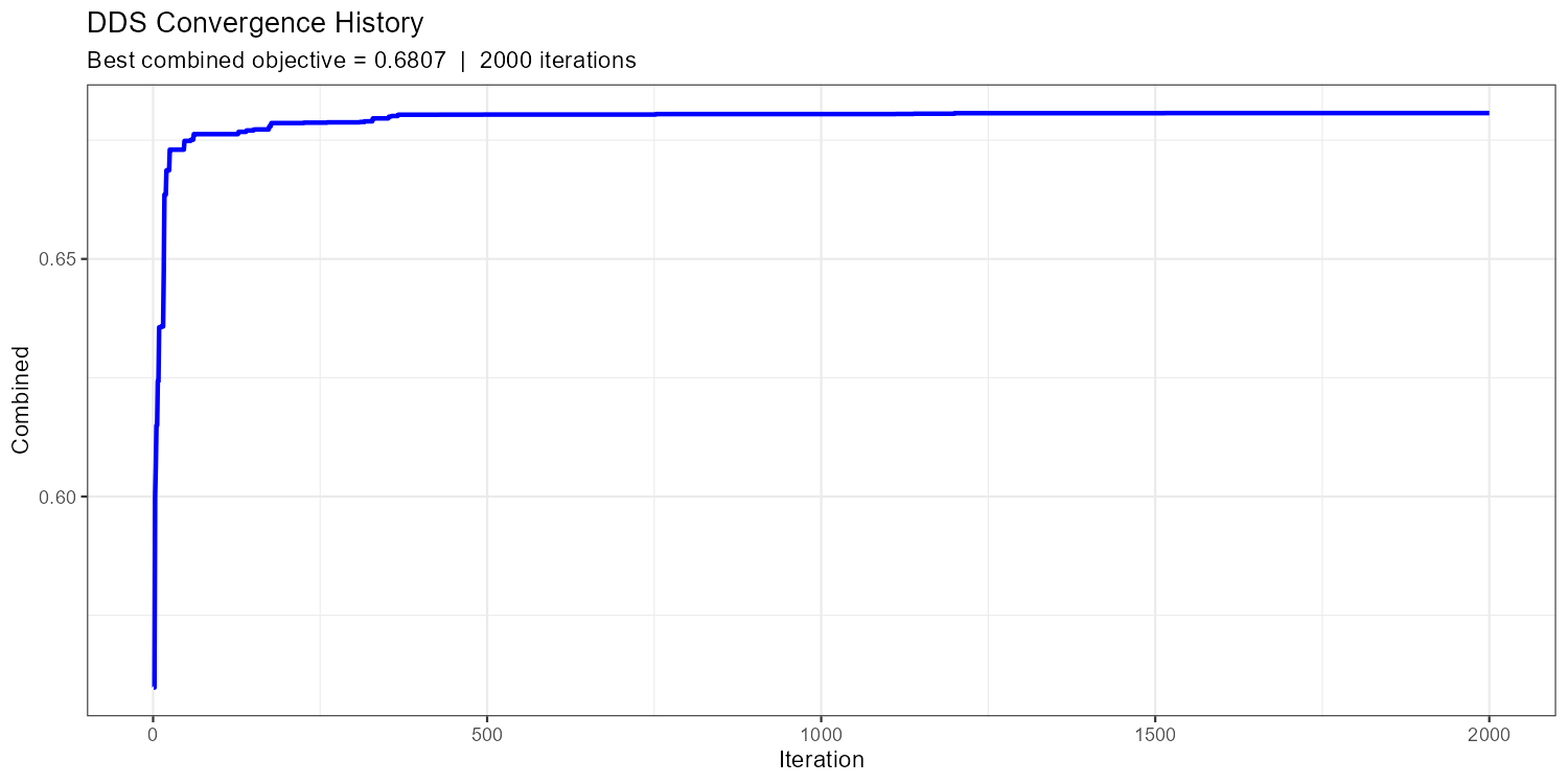
max_iter.
A healthy convergence curve drops steeply in the first ~20% of iterations and then flattens with occasional improvements. If the curve is still clearly declining at the end, increase max_iter. If it flattened after fewer than 100 iterations, you may have too few free parameters or too narrow bounds.
SCE-UA as an Alternative
NoteSCE-UA — Shuffled Complex Evolution
The CoseRo package also provides optimize_cosero_sce(), which implements the Shuffled Complex Evolution algorithm (Duan et al., 1993). SCE-UA maintains a population of parameter sets (complexes) that evolve simultaneously through competitive evolution. Unlike DDS, SCE-UA has a formal stopping criterion: it terminates early if the objective function no longer improves meaningfully, which can save evaluations when convergence is fast. The trade-off is that it requires a larger minimum budget (typically 2000–5000 evaluations) to adequately explore the parameter space with multiple complexes.
Consider SCE-UA if:
- You want automatic stopping based on convergence rather than a fixed iteration budget
- DDS results vary substantially between runs (suggesting the search space is not well explored)
- You have a fast model and can afford a larger evaluation budget
Show/hide: SCE-UA call
result_sce <- optimize_cosero_sce(
  cosero_path       = project_path,
  par_bounds        = par_bounds,        # same bounds as DDS
  target_subbasins  = subbasins,
  metric            = "NSE",             # single metric for SCE-UA
  aggregation       = "mean",
  subbasin_weights  = c(0.5, 0.3, 0.2),
  defaults_settings = list(
    STARTDATE  = "2004 1 1 0 0",
    ENDDATE    = "2024 12 31 0 0",
    SPINUP     = 365,
    OUTPUTTYPE = 1,
    PARAFILE        = "para_ini.txt",
    statevar_source = 2                  # warm start: reuse state variables between iterations
  ),
  maxn    = 2000,   # maximum number of model evaluations
  ngs     = 3,      # number of complexes; more = wider global search, more evaluations
  verbose = TRUE
)
Part 4: Calibration Results & Full-Period Run
NoteWhat you’ll learn
Export the optimised parameter file, do a quick visual check comparing the initial and calibrated hydrograph, then run the full data period with full output (OUTPUTTYPE = 3) for in-depth analysis.
Exporting the Optimised Parameter File
The CoseRo optimisation functions automatically write the best parameter set to the project’s output directory. Use export_cosero_optimization() to also save the full optimisation history and summary to a results folder for reproducibility:
results_dir <- file.path(project_path, "calibration_results")
dir.create(results_dir, showWarnings = FALSE, recursive = TRUE)

# Exports: parameter file, history CSV, summary text
export_cosero_optimization(result_dds,
                           output_dir = file.path(results_dir, "DDS_NSE_KGE"))

# Path to the saved calibrated parameter file
par_file_cal <- result_dds$optimized_par_file
cat("Calibrated parameter file saved to:\n", par_file_cal, "\n")
Initial vs. Calibrated Hydrograph
Before running the full period, do a quick sanity check: compare the initial and calibrated hydrographs over the calibration period to confirm the optimisation improved performance.
Show/hide: Initial vs. calibrated comparison
# Re-run with initial parameters for comparison
result_ini <- run_cosero(
  project_path      = project_path,
  defaults_settings = list(
    STARTDATE  = "2004 1 1 0 0",
    ENDDATE    = "2024 12 31 0 0",
    SPINUP     = 365,
    OUTPUTTYPE = 1,
    PARAFILE   = "para_ini.txt",
    statevar_source = 2
  )
)

# Copy calibrated parameter file to input/ so COSERO can find it
par_file_cal_input <- file.path(project_path, "input", basename(par_file_cal))
file.copy(par_file_cal, par_file_cal_input, overwrite = TRUE)

# Re-run with calibrated parameters
result_cal_check <- run_cosero(
  project_path      = project_path,
  defaults_settings = list(
    STARTDATE  = "2004 1 1 0 0",
    ENDDATE    = "2024 12 31 0 0",
    SPINUP     = 365,
    OUTPUTTYPE = 1,
    PARAFILE   = basename(par_file_cal_input),
    statevar_source = 2
  )
)

sb_id    <- sprintf("%04d", as.integer(target_subbasin))
spinup   <- 365
idx      <- (spinup + 1):nrow(result_ini$output_data$runoff)
run_date <- result_ini$output_data$runoff$DateTime[idx]

nse_ini <- extract_run_metrics(result_ini,       target_subbasin, "NSE")
nse_cal <- extract_run_metrics(result_cal_check, target_subbasin, "NSE")

df_comp <- data.frame(
  Date       = as.Date(run_date),
  Observed   = result_ini$output_data$runoff[[paste0("QOBS_", sb_id)]][idx],
  Initial    = result_ini$output_data$runoff[[paste0("QSIM_", sb_id)]][idx],
  Calibrated = result_cal_check$output_data$runoff[[paste0("QSIM_", sb_id)]][idx]
) |>
  pivot_longer(-Date, names_to = "Series", values_to = "Q") |>
  mutate(Q = ifelse(Q < 0, NA_real_, Q))   # replace negative artefacts with NA

df_comp$Series <- factor(df_comp$Series,
                         levels = c("Observed", "Initial", "Calibrated"))

p_comp <- ggplot(df_comp, aes(x = Date, y = Q, colour = Series)) +
  geom_line(linewidth = 0.3, alpha = 0.8) +
  scale_colour_manual(values = c(Observed = "black", Initial = "grey60",
                                  Calibrated = "#C0392B")) +
  scale_x_date(expand = expansion(add = 30)) +
  labs(
    title    = paste("Subbasin", target_subbasin, "— Initial vs. Calibrated"),
    subtitle = sprintf("NSE:  Initial = %.3f  →  Calibrated = %.3f", nse_ini, nse_cal),
    x = NULL, y = expression(Q~"["*m^3*s^{-1}*"]"), colour = NULL
  ) +
  theme_bw() + theme(legend.position = "top",
                     axis.title = element_text(size = 12))

print(p_comp)
ggsave(file.path(plot_dir, paste0("hydro_initial_vs_cal_NB", target_subbasin, ".png")),
       p_comp, width = 14, height = 5, dpi = 150)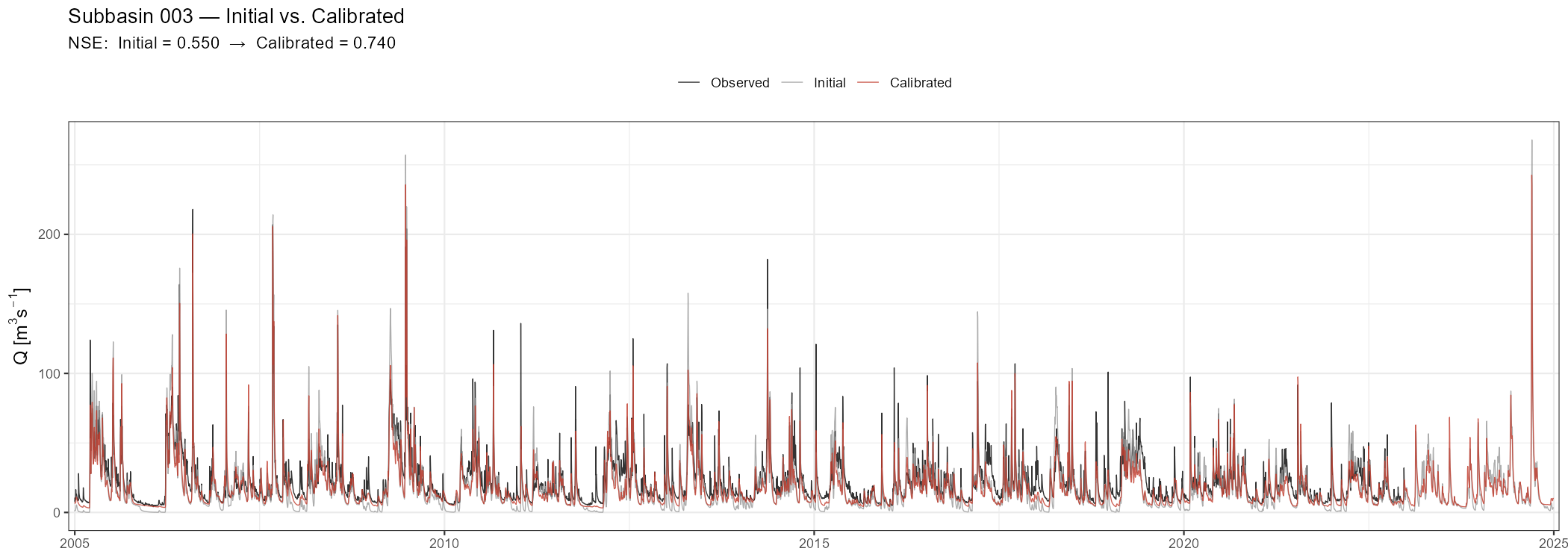
Full-Period Run with OUTPUTTYPE = 3
Once you have confirmed the calibration improved performance, run the full available data period with all outputs enabled. This single run produces all the data needed for Parts 5–8.
result <- run_cosero(
  project_path      = project_path,
  defaults_settings = list(
    STARTDATE       = "1991 1 1 0 0",         # full period including spin-up
    ENDDATE         = "2024 12 31 0 0",
    SPINUP          = 365,                    # first year excluded from all metrics
    OUTPUTTYPE      = 3,                      # full output: all files (see table below)
    PARAFILE        = basename(par_file_cal_input), # calibrated parameter file (copied to input/)
    statevar_source = 1                       # cold start
  )
)

out    <- result$output_data

spinup <- 365
out$runoff             <- out$runoff[(spinup + 1):nrow(out$runoff), ]
out$runoff_components  <- out$runoff_components[(spinup + 1):nrow(out$runoff_components), ]
out$water_balance      <- out$water_balance[(spinup + 1):nrow(out$water_balance), ]

runoff <- out$runoff
runoff[runoff < 0] <- NA
OUTPUTTYPE = 3 activates all COSERO output files. To see exactly what is written, browse your project’s output folder and inspect the individual files — the column names in each file correspond directly to the named elements in the out list returned by read_cosero_output().
Quick Visual Check with the Shiny App
Before the detailed analysis below, launch the CoseRo Shiny app for an interactive first look at the calibrated results. Refer to Module 3, Part 2 for a detailed description of the app’s five tabs.
launch_cosero_app(project_path)Part 5: Performance Assessment — Calibration vs. Validation
NoteWhat you’ll learn
Compute NSE, KGE, and BETA for the calibration and validation periods separately, print a formatted comparison table, and interpret what the numbers say about model transferability.
Helper Functions
Define the metric functions once here; they are reused in the analysis plots further below.
calc_nse <- function(obs, sim) {
  valid <- !is.na(obs) & !is.na(sim)
  obs <- obs[valid]; sim <- sim[valid]
  1 - sum((obs - sim)^2) / sum((obs - mean(obs))^2)
}

calc_kge <- function(obs, sim) {
  valid <- !is.na(obs) & !is.na(sim)
  obs <- obs[valid]; sim <- sim[valid]
  r     <- cor(sim, obs)
  alpha <- sd(sim) / sd(obs)
  beta  <- mean(sim) / mean(obs)
  1 - sqrt((r - 1)^2 + (alpha - 1)^2 + (beta - 1)^2)
}

calc_beta <- function(obs, sim) {
  valid <- !is.na(obs) & !is.na(sim)
  mean(sim[valid]) / mean(obs[valid])   # volume ratio; 1.0 = unbiased
}
Calibration / Validation / Full-Period Metrics
dates    <- as.Date(runoff$DateTime)

performance <- data.frame()

for (sb in subbasins) {
  sb_id    <- sprintf("%04d", as.integer(sb))
  qobs_col <- paste0("QOBS_", sb_id)
  qsim_col <- paste0("QSIM_", sb_id)

  obs_full <- runoff[[qobs_col]]
  sim_full <- runoff[[qsim_col]]

  periods <- list(
    Calibration = dates >= cal_start & dates <= cal_end,
    Validation  = dates >= val_start & dates <= val_end,
    Full        = rep(TRUE, length(dates))
  )

  for (period_name in names(periods)) {
    idx_p <- periods[[period_name]]
    performance <- rbind(performance, data.frame(
      Subbasin = sb,
      Period   = period_name,
      NSE      = round(calc_nse(obs_full[idx_p], sim_full[idx_p]), 3),
      KGE      = round(calc_kge(obs_full[idx_p], sim_full[idx_p]), 3),
      BETA     = round(calc_beta(obs_full[idx_p], sim_full[idx_p]), 3)
    ))
  }
}

print(performance)| Subbasin | Period | NSE | KGE | BETA |
|---|---|---|---|---|
| 001 | Calibration | 0.667 | 0.823 | 1.066 |
| 001 | Validation | 0.678 | 0.823 | 1.054 |
| 001 | Full | 0.676 | 0.831 | 1.058 |
| 002 | Calibration | 0.581 | 0.577 | 1.195 |
| 002 | Validation | 0.510 | 0.473 | 1.239 |
| 002 | Full | 0.550 | 0.532 | 1.214 |
| 003 | Calibration | 0.731 | 0.796 | 0.829 |
| 003 | Validation | 0.772 | 0.844 | 0.882 |
| 003 | Full | 0.751 | 0.817 | 0.851 |
ImportantInterpreting the calibration–validation comparison
A small drop in validation NSE (0.02–0.06) is normal and expected — the calibration period was the data the optimiser saw. A large drop (>0.10) warrants investigation:
- Different hydroclimatic regime? If the two periods differ substantially in wetness or temperature, the same parameters may not generalise.
- Parameter overfitting? Too many free parameters relative to the information content of the calibration data.
- Non-stationarity? Land use change, vegetation dynamics, or long-term climate trends between the two periods.
- BETA >> 1 in validation? The model is running too wet — a common symptom of input undercatch in the calibration period being compensated by PCOR.
Always report both periods transparently.
Part 6: Hydrograph, Residuals & Seasonal Analysis
NoteWhat you’ll learn
Visualise the calibrated model’s performance across multiple diagnostic angles: the full hydrograph with calibration/validation boundary marked, event zooms, scatter plot, flow duration curve, residuals, monthly regime, and seasonal performance breakdown.
Full-Period Hydrograph
The full-period hydrograph is the primary visual diagnostic. A vertical dashed line marks the transition from calibration to validation.
Show/hide: Full-period hydrograph
sb_id    <- sprintf("%04d", as.integer(target_subbasin))

df_hydro <- data.frame(
  Date      = as.Date(runoff$DateTime),
  Observed  = runoff[[paste0("QOBS_", sb_id)]],
  Simulated = runoff[[paste0("QSIM_", sb_id)]]
)

nse_full <- calc_nse(df_hydro$Observed, df_hydro$Simulated)
kge_full <- calc_kge(df_hydro$Observed, df_hydro$Simulated)

p_full <- ggplot(df_hydro, aes(x = Date)) +
  geom_line(aes(y = Observed,  colour = "Observed"),  linewidth = 0.3, alpha = 0.8) +
  geom_line(aes(y = Simulated, colour = "Simulated"), linewidth = 0.3, alpha = 0.8) +
  geom_vline(xintercept = cal_start,
             linetype = "dashed", colour = "grey40", linewidth = 0.5) +
  annotate("text", x = cal_start + 200,
           y = max(df_hydro$Observed, na.rm = TRUE) * 0.92,
           label = "Calibration", hjust = 0, size = 3, colour = "grey40") +
  annotate("text", x = min(df_hydro$Date) + 200,
           y = max(df_hydro$Observed, na.rm = TRUE) * 0.92,
           label = "Validation", hjust = 0, size = 3, colour = "grey40") +
  scale_colour_manual(values = c(Observed = "black", Simulated = "#C0392B")) +
  scale_x_date(expand = expansion(add = 30)) +
  labs(
    title    = paste("Subbasin", target_subbasin, "— Full Period"),
    subtitle = sprintf("NSE = %.3f  |  KGE = %.3f  |  Calibrated parameters",
                       nse_full, kge_full),
    x = NULL, y = expression(Q~"["*m^3*s^{-1}*"]"), colour = NULL
  ) +
  theme_bw() + theme(legend.position = "top",
                     axis.title = element_text(size = 12))

print(p_full)
ggsave(file.path(plot_dir, paste0("hydro_full_NB", target_subbasin, ".png")),
       p_full, width = 14, height = 5, dpi = 150)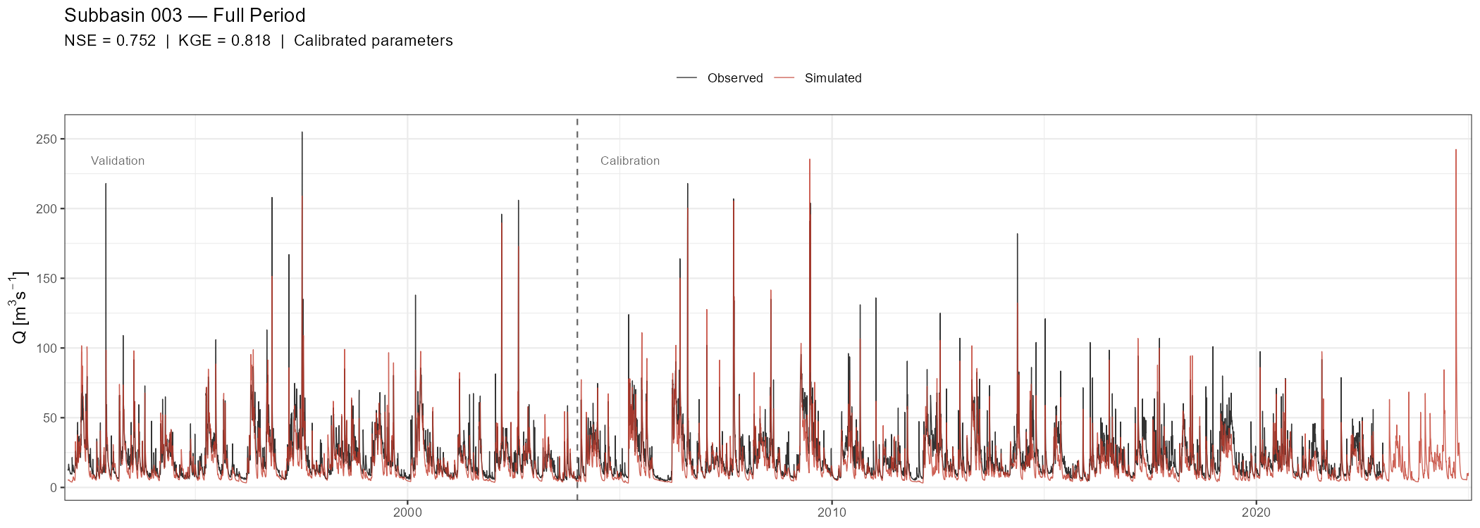
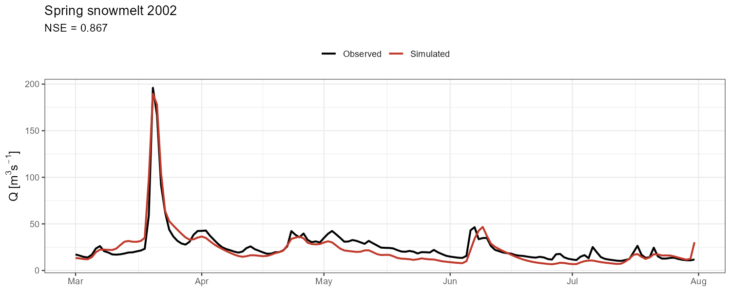
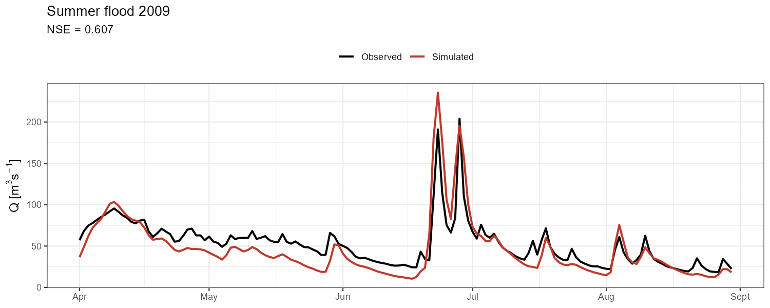
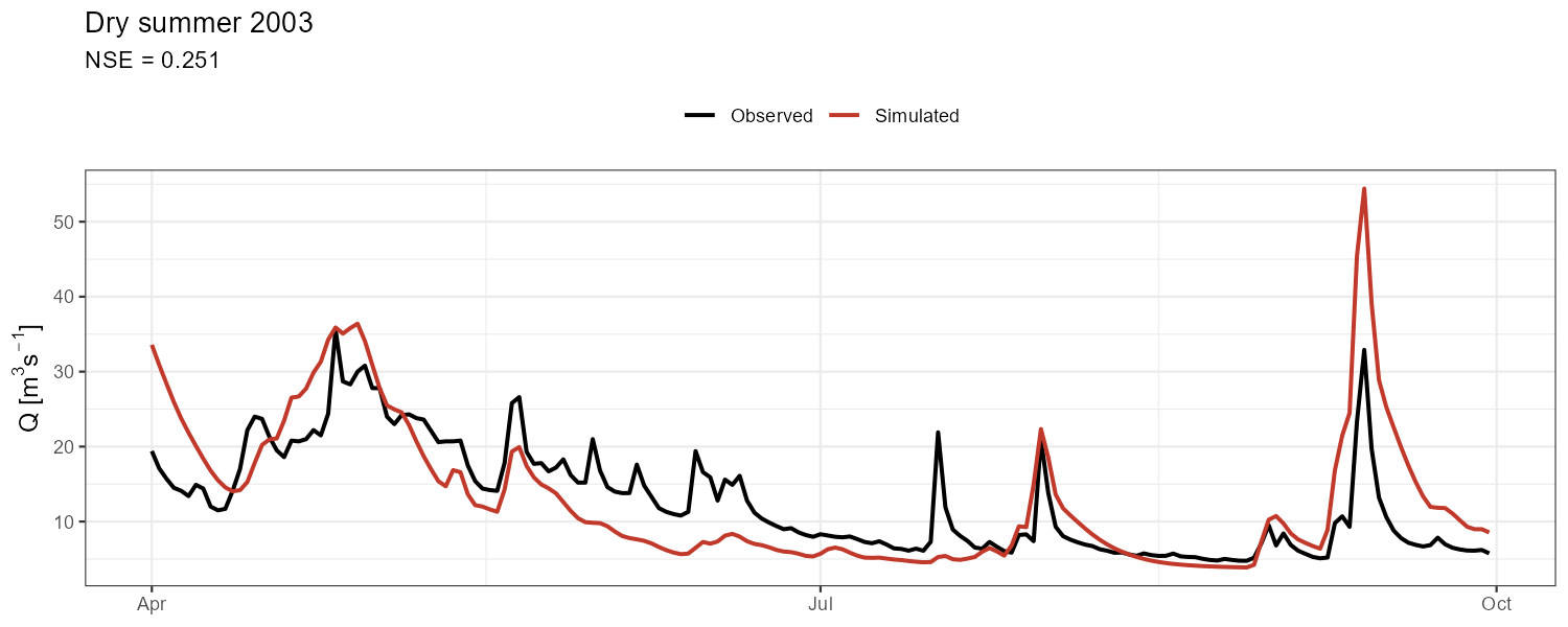
Event Zooms
Aggregate metrics can mask compensating errors. Zoom into contrasting events to check timing, peak magnitude, and recession behaviour separately.
Show/hide: Event zoom code
# Adjust event dates to your catchment and data period
events <- list(
  "Spring snowmelt 2002" = c(as.Date("2002-03-01"), as.Date("2002-07-31")),
  "Summer flood 2009"    = c(as.Date("2009-04-01"), as.Date("2009-08-30")),
  "Dry summer 2003"      = c(as.Date("2003-04-01"), as.Date("2003-09-30"))
)

for (event_name in names(events)) {
  d1 <- events[[event_name]][1]; d2 <- events[[event_name]][2]
  df_ev <- df_hydro |> filter(Date >= d1 & Date <= d2)
  if (nrow(df_ev) < 10) next

  nse_ev <- calc_nse(df_ev$Observed, df_ev$Simulated)

  p_ev <- ggplot(df_ev, aes(x = Date)) +
    geom_line(aes(y = Observed,  colour = "Observed"),  linewidth = 0.9) +
    geom_line(aes(y = Simulated, colour = "Simulated"), linewidth = 0.9) +
    scale_colour_manual(values = c(Observed = "black", Simulated = "#C0392B")) +
    labs(title    = event_name,
         subtitle = sprintf("NSE = %.3f", nse_ev),
         x = NULL, y = expression(Q~"["*m^3*s^{-1}*"]"), colour = NULL) +
    theme_bw() + theme(legend.position = "top",
                       axis.title = element_text(size = 12))
  print(p_ev)
  ggsave(file.path(plot_dir,
                   paste0("event_", gsub("[^A-Za-z0-9]", "_", event_name), ".png")),
         p_ev, width = 10, height = 4, dpi = 150)
}
Scatter Plot and Flow Duration Curve
Show/hide: Scatter plot and FDC
# Observed vs. simulated scatter (1:1 line = perfect fit)
q_lim <- quantile(df_hydro$Observed, 0.995, na.rm = TRUE)
p_scatter <- ggplot(df_hydro, aes(x = Observed, y = Simulated)) +
  geom_point(alpha = 0.12, size = 0.5, colour = "#5E4B8B") +
  geom_abline(intercept = 0, slope = 1, colour = "grey60", linetype = "dashed", linewidth = 0.5) +
  geom_smooth(method = "lm", se = TRUE, colour = "#C0392B", linewidth = 0.3) +  # thin lm line
  coord_fixed(xlim = c(0, q_lim), ylim = c(0, q_lim)) +
  labs(title = paste("Subbasin", target_subbasin),
       x = expression("Observed Q ["*m^3*s^{-1}*"]"),
       y = expression("Simulated Q ["*m^3*s^{-1}*"]")) +
  theme_bw()
print(p_scatter)
ggsave(file.path(plot_dir, paste0("scatter_NB", target_subbasin, ".png")),
       p_scatter, width = 4, height = 4, dpi = 150)

# Flow duration curve (log scale)
calc_fdc <- function(Q) {
  Q_sorted <- sort(Q[!is.na(Q)], decreasing = TRUE)
  data.frame(
    Exceedance = seq_along(Q_sorted) / (length(Q_sorted) + 1) * 100,
    Q          = Q_sorted
  )
}

fdc_df <- bind_rows(
  calc_fdc(df_hydro$Observed)  |> mutate(Series = "Observed"),
  calc_fdc(df_hydro$Simulated) |> mutate(Series = "Simulated")
)

p_fdc <- ggplot(fdc_df, aes(x = Exceedance, y = Q, colour = Series)) +
  geom_line(linewidth = 0.7) + scale_y_log10() +
  scale_colour_manual(values = c(Observed = "black", Simulated = "#C0392B")) +
  scale_x_continuous(
    name = "Exceedance probability (%)",
    sec.axis = sec_axis(~ . / 100 * 365, name = "Days per year exceeded",
                        breaks = c(1, 7, 30, 91, 182, 274, 365))
  ) +
  labs(title = paste("Flow Duration Curve — Subbasin", target_subbasin),
       y = expression("Q ["*m^3*s^{-1}*"]  (log scale)"), colour = NULL) +
  theme_bw() + theme(legend.position = "top")
print(p_fdc)
ggsave(file.path(plot_dir, paste0("fdc_NB", target_subbasin, ".png")),
       p_fdc, width = 8, height = 5, dpi = 150)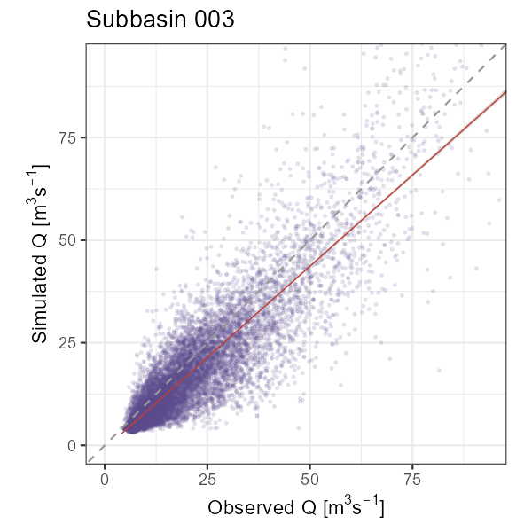
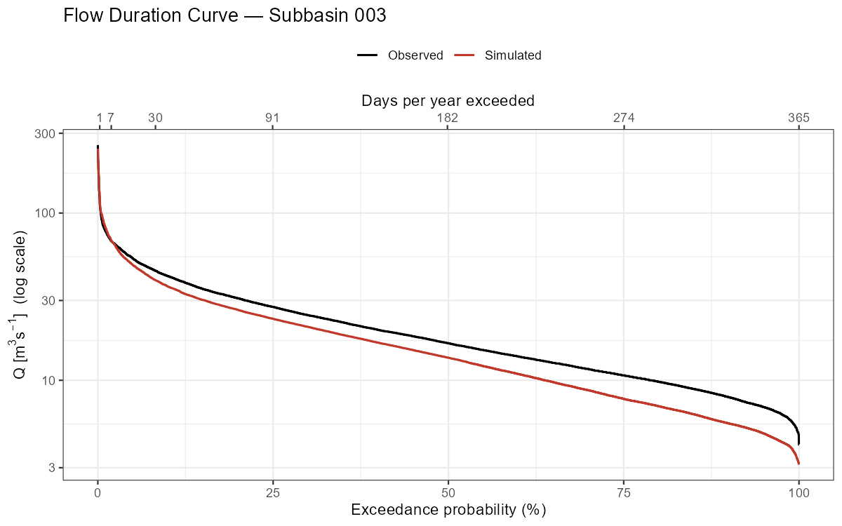
The flow duration curve is useful for diagnosing systematic biases: a mismatch at high exceedance probabilities indicates a baseflow problem, while a mismatch at low exceedance probabilities indicates peak flow errors.
Residual Diagnostics
Residuals (simulated − observed) should scatter randomly around zero without trends or seasonal cycles. Any systematic pattern is a signal of model deficiency.
Show/hide: Residual plots
df_hydro <- df_hydro |> mutate(Residual = Simulated - Observed)

p_resid <- ggplot(df_hydro, aes(x = Date, y = Residual)) +
  geom_line(linewidth = 0.2, alpha = 0.4, colour = "grey40") +
  geom_hline(yintercept = 0, colour = "red", linetype = "dashed") +
  geom_smooth(method = "loess", span = 0.08, colour = "#5E4B8B", se = FALSE) +
  geom_vline(xintercept = cal_start,
             linetype = "dashed", colour = "grey50", linewidth = 0.5) +
  scale_x_date(expand = expansion(add = 30)) +
  labs(title = paste("Residuals — Subbasin", target_subbasin),
       subtitle = "LOESS smoother highlights systematic bias trends",
       x = NULL, y = expression("Residual ["*m^3*s^{-1}*"]")) +
  theme_bw() + theme(axis.title = element_text(size = 13),
                     axis.text  = element_text(size = 11))
print(p_resid)
ggsave(file.path(plot_dir, paste0("residuals_NB", target_subbasin, ".png")),
       p_resid, width = 14, height = 4, dpi = 150)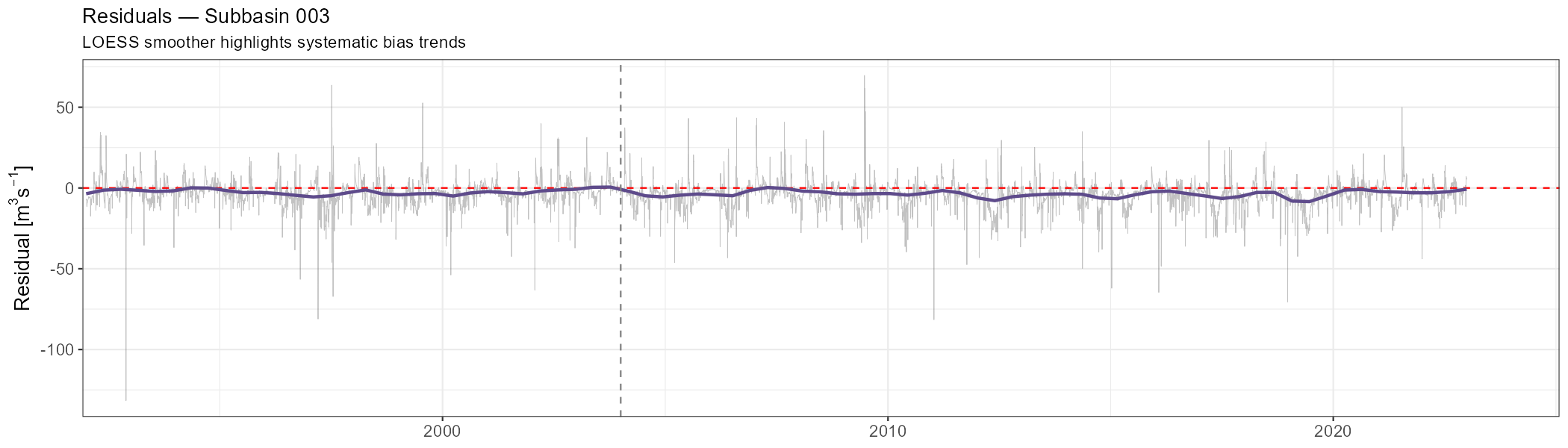
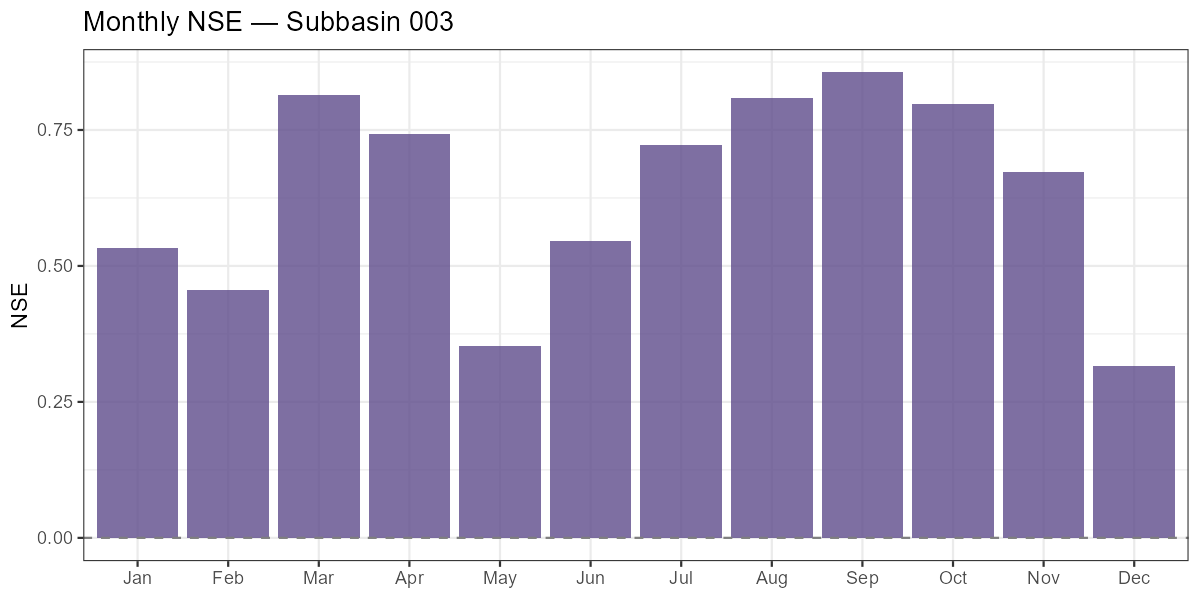
Monthly Discharge Regime
The mean monthly regime shows whether the model captures the seasonal timing of discharge — critical for snow-dominated catchments where the melt peak must be reproduced.
Show/hide: Monthly regime and NSE
monthly_stats <- df_hydro |>
  mutate(Month = as.integer(format(Date, "%m"))) |>
  group_by(Month) |>
  summarise(
    Obs_mean = mean(Observed,  na.rm = TRUE),
    Sim_mean = mean(Simulated, na.rm = TRUE),
    Obs_q25  = quantile(Observed, 0.25, na.rm = TRUE),
    Obs_q75  = quantile(Observed, 0.75, na.rm = TRUE),
    NSE_mon  = calc_nse(Observed, Simulated),
    .groups  = "drop"
  )

# Mean monthly regime
p_regime <- ggplot(monthly_stats, aes(x = Month)) +
  geom_ribbon(aes(ymin = Obs_q25, ymax = Obs_q75), fill = "grey80", alpha = 0.5) +
  geom_line(aes(y = Obs_mean, colour = "Observed"),  linewidth = 1.2) +
  geom_line(aes(y = Sim_mean, colour = "Simulated"), linewidth = 1.2) +
  scale_x_continuous(breaks = 1:12, labels = month.abb) +
  scale_colour_manual(values = c(Observed = "black", Simulated = "#C0392B")) +
  labs(title    = paste("Mean Monthly Regime — Subbasin", target_subbasin),
       subtitle = "Ribbon = observed interquartile range",
       x = NULL, y = expression("Mean Q ["*m^3*s^{-1}*"]"), colour = NULL) +
  theme_bw() + theme(legend.position = "top")
print(p_regime)
ggsave(file.path(plot_dir, paste0("regime_NB", target_subbasin, ".png")),
       p_regime, width = 8, height = 5, dpi = 150)

# Monthly NSE bar chart
p_mon_nse <- ggplot(monthly_stats, aes(x = factor(Month, labels = month.abb), y = NSE_mon)) +
  geom_col(fill = "#5E4B8B", alpha = 0.8) +
  geom_hline(yintercept = 0, linetype = "dashed", colour = "grey50") +
  labs(title = paste("Monthly NSE — Subbasin", target_subbasin),
       x = NULL, y = "NSE") +
  theme_bw()
print(p_mon_nse)
ggsave(file.path(plot_dir, paste0("monthly_nse_NB", target_subbasin, ".png")),
       p_mon_nse, width = 8, height = 4, dpi = 150)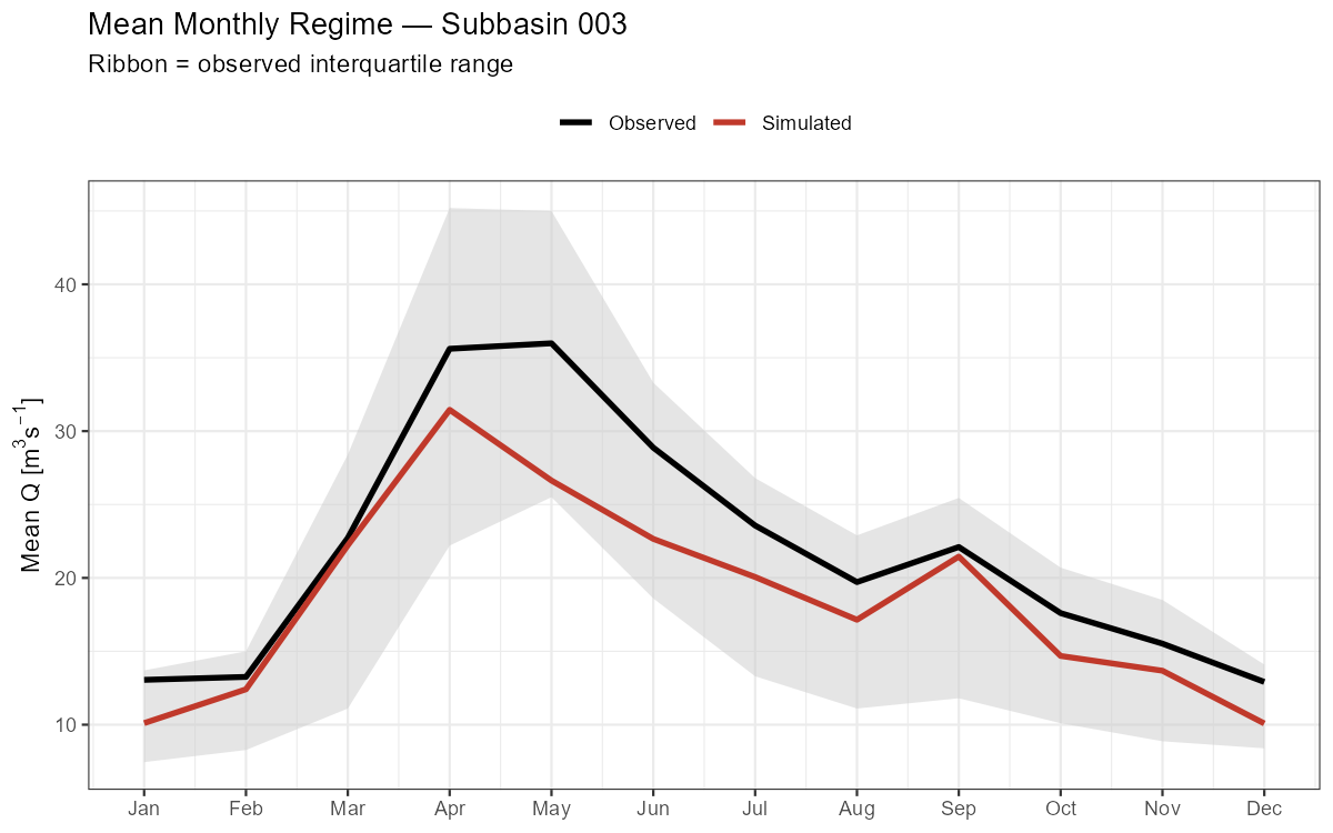
Seasonal Performance Breakdown
Show/hide: Seasonal NSE/KGE breakdown
seasonal <- df_hydro |>
  mutate(Season = case_when(
    as.integer(format(Date, "%m")) %in% c(12, 1, 2) ~ "DJF (Winter)",
    as.integer(format(Date, "%m")) %in% c(3, 4, 5)  ~ "MAM (Spring)",
    as.integer(format(Date, "%m")) %in% c(6, 7, 8)  ~ "JJA (Summer)",
    TRUE                                              ~ "SON (Autumn)"
  )) |>
  group_by(Season) |>
  summarise(
    NSE  = calc_nse(Observed, Simulated),
    KGE  = calc_kge(Observed, Simulated),
    BETA = calc_beta(Observed, Simulated),
    .groups = "drop"
  )

print(seasonal)

p_seasonal <- seasonal |>
  pivot_longer(c(NSE, KGE), names_to = "Metric", values_to = "Value") |>
  ggplot(aes(x = Season, y = Value, fill = Metric)) +
  geom_col(position = "dodge", alpha = 0.85) +
  geom_hline(yintercept = 0, linetype = "dashed", colour = "grey50") +
  scale_fill_manual(values = c(NSE = "#5E4B8B", KGE = "#4CAF71")) +
  labs(title = paste("Seasonal Performance — Subbasin", target_subbasin),
       x = NULL, y = "Metric value", fill = NULL) +
  theme_bw() + theme(legend.position = "top")
print(p_seasonal)
ggsave(file.path(plot_dir, paste0("seasonal_perf_NB", target_subbasin, ".png")),
       p_seasonal, width = 8, height = 5, dpi = 150)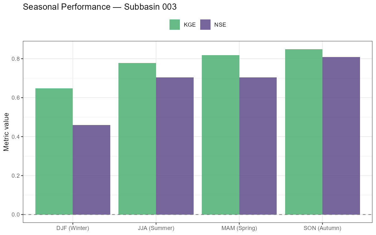
Months with low or negative monthly NSE indicate where the model struggles most. In alpine catchments, poor spring NSE often signals incorrect snow accumulation or melt timing, while poor summer NSE can indicate missing soil moisture dynamics during dry spells.
Part 7: Water Balance & Runoff Components
NoteWhat you’ll learn
Decompose the simulated water balance into precipitation, evapotranspiration, runoff, and storage change. Break discharge into its three routing components, inspect storage time series, and verify that annual water balance closure is physically plausible.
Runoff Components
COSERO routes water through three parallel storage reservoirs, each draining at a different rate. The output runoff_components contains the depth-equivalent contributions:
| Variable | Description |
|---|---|
QAB123GEB |
Total simulated runoff depth (all three components) |
QAB23GEB |
Subsurface runoff (interflow + baseflow) |
QAB3GEB |
Baseflow only |
Surface runoff is derived as QAB123 − QAB23, interflow as QAB23 − QAB3.
Show/hide: Annual runoff components
rc    <- out$runoff_components
sb_id <- sprintf("%04d", as.integer(target_subbasin))

df_rc <- data.frame(
  Date      = as.Date(rc$DateTime),
  Total     = rc[[paste0("QAB123GEB_", sb_id)]],
  Subsurface = rc[[paste0("QAB23GEB_",  sb_id)]],
  Baseflow  = rc[[paste0("QAB3GEB_",   sb_id)]]
) |>
  mutate(
    Surface   = Total - Subsurface,
    Interflow = Subsurface - Baseflow
  )

annual_rc <- df_rc |>
  mutate(Year = as.integer(format(Date, "%Y"))) |>
  group_by(Year) |>
  summarise(Surface   = sum(Surface,   na.rm = TRUE),
            Interflow = sum(Interflow, na.rm = TRUE),
            Baseflow  = sum(Baseflow,  na.rm = TRUE),
            .groups = "drop") |>
  pivot_longer(-Year, names_to = "Component", values_to = "mm")

annual_rc$Component <- factor(annual_rc$Component,
                               levels = c("Surface", "Interflow", "Baseflow"))

p_rc <- ggplot(annual_rc, aes(x = Year, y = mm, fill = Component)) +
  geom_col() +
  scale_fill_manual(values = c(Surface = "#E67E3C", Interflow = "#5E4B8B",
                                Baseflow = "#4CAF71")) +
  labs(title = paste("Annual Runoff Components — Subbasin", target_subbasin),
       x = NULL, y = "Runoff depth (mm/year)", fill = NULL) +
  theme_bw() + theme(legend.position = "top",
                     axis.title = element_text(size = 12))
print(p_rc)
ggsave(file.path(plot_dir, paste0("runoff_components_NB", target_subbasin, ".png")),
       p_rc, width = 10, height = 5, dpi = 150)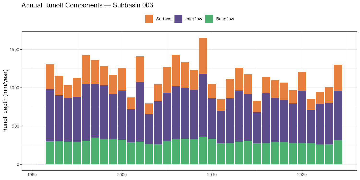
Storage Time Series
Inspecting the model’s internal storage states confirms whether snow accumulation, soil moisture depletion, and groundwater recharge are physically plausible — independent of the discharge fit.
Show/hide: Storage time series
wb    <- out$water_balance

df_stor <- data.frame(
  Date             = as.Date(wb$DateTime),
  `Soil (BW0, mm)` = wb[[paste0("BW0GEB_", sb_id)]],
  `Groundwater (BW3, mm)` = wb[[paste0("BW3GEB_", sb_id)]],
  `Snow (SWW, mm)` = wb[[paste0("SWWGEB_",  sb_id)]],
  check.names = FALSE
) |> pivot_longer(-Date, names_to = "Variable", values_to = "mm")

p_stor <- ggplot(df_stor, aes(x = Date, y = mm, colour = Variable)) +
  geom_line(linewidth = 0.3) +
  facet_wrap(~Variable, ncol = 1, scales = "free_y") +
  scale_colour_manual(values = c(
    "Soil (BW0, mm)"         = "#E67E3C",
    "Groundwater (BW3, mm)"  = "#5E4B8B",
    "Snow (SWW, mm)"         = "#00BFFF"
  )) +
  labs(title = paste("Storage States — Subbasin", target_subbasin),
       x = NULL, y = "mm") +
  theme_bw() + theme(legend.position = "none",
                     strip.background = element_blank(),
                     strip.text = element_text(face = "bold"),
                     axis.title = element_text(size = 12))
print(p_stor)
ggsave(file.path(plot_dir, paste0("storages_NB", target_subbasin, ".png")),
       p_stor, width = 14, height = 8, dpi = 150)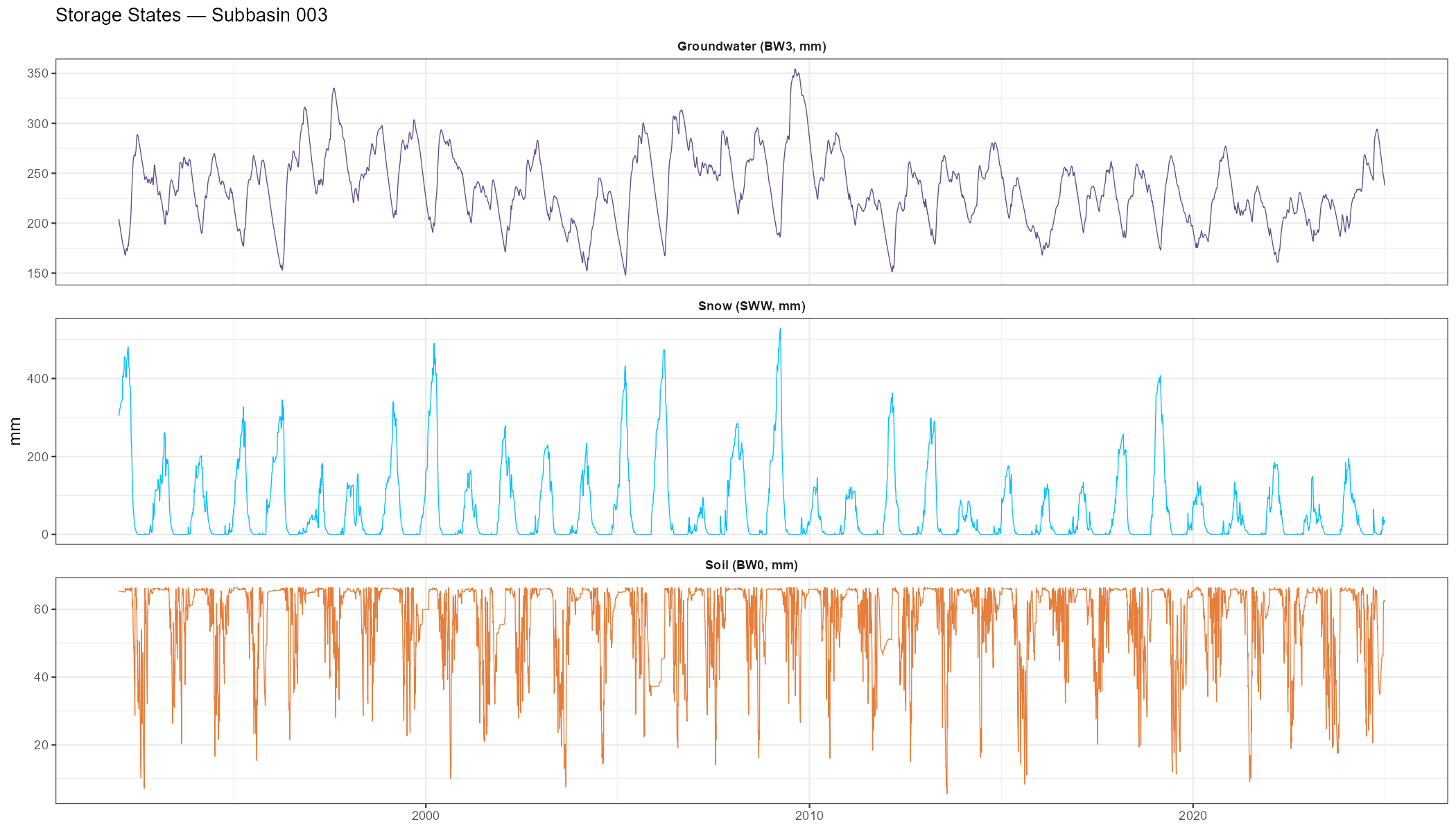
Annual Water Balance
The annual water balance closure check — \(P - ET - Q \approx \Delta S\) — is a fundamental model diagnostic. Large systematic residuals indicate errors in input data or model structure that calibration has masked.
Show/hide: Annual water balance table and plot
wb_sub <- wb

wb_annual <- wb_sub |>
  mutate(
    Date = as.Date(DateTime),
    Year = as.integer(format(Date, "%Y"))
  ) |>
  group_by(Year) |>
  summarise(
    P   = sum(.data[[paste0("PGEB_",     sb_id)]], na.rm = TRUE),
    ET  = sum(.data[[paste0("ETAGEB_",   sb_id)]], na.rm = TRUE),
    Q   = sum(.data[[paste0("QABGEB_",   sb_id)]], na.rm = TRUE),
    dS  = (.data[[paste0("BW0GEB_",  sb_id)]][n()] +
           .data[[paste0("BW3GEB_",  sb_id)]][n()] +
           .data[[paste0("SWWGEB_",  sb_id)]][n()]) -
          (.data[[paste0("BW0GEB_",  sb_id)]][1]   +
           .data[[paste0("BW3GEB_",  sb_id)]][1]   +
           .data[[paste0("SWWGEB_",  sb_id)]][1]),
    .groups = "drop"
  ) |>
  mutate(
    Residual  = P - ET - Q - dS,
    Q_ratio   = round(Q / P * 100, 1),
    ET_ratio  = round(ET / P * 100, 1)
  )

print(wb_annual)

wb_long <- wb_annual |>
  select(Year, P, ET, Q) |>
  pivot_longer(-Year, names_to = "Component", values_to = "mm")
wb_long$Component <- factor(wb_long$Component,
                             levels = c("P", "ET", "Q"),
                             labels = c("Precipitation", "Evapotranspiration", "Runoff"))

p_wb <- ggplot(wb_long, aes(x = Year, y = mm, fill = Component)) +
  geom_col(position = "dodge") +
  scale_fill_manual(values = c(Precipitation = "#0066CC",
                                Evapotranspiration = "#E67E3C", Runoff = "#4CAF71")) +
  labs(title = paste("Annual Water Balance — Subbasin", target_subbasin),
       x = NULL, y = "mm/year", fill = NULL) +
  theme_bw() + theme(legend.position = "top",
                     axis.title = element_text(size = 12))
print(p_wb)
ggsave(file.path(plot_dir, paste0("annual_wb_NB", target_subbasin, ".png")),
       p_wb, width = 10, height = 5, dpi = 150)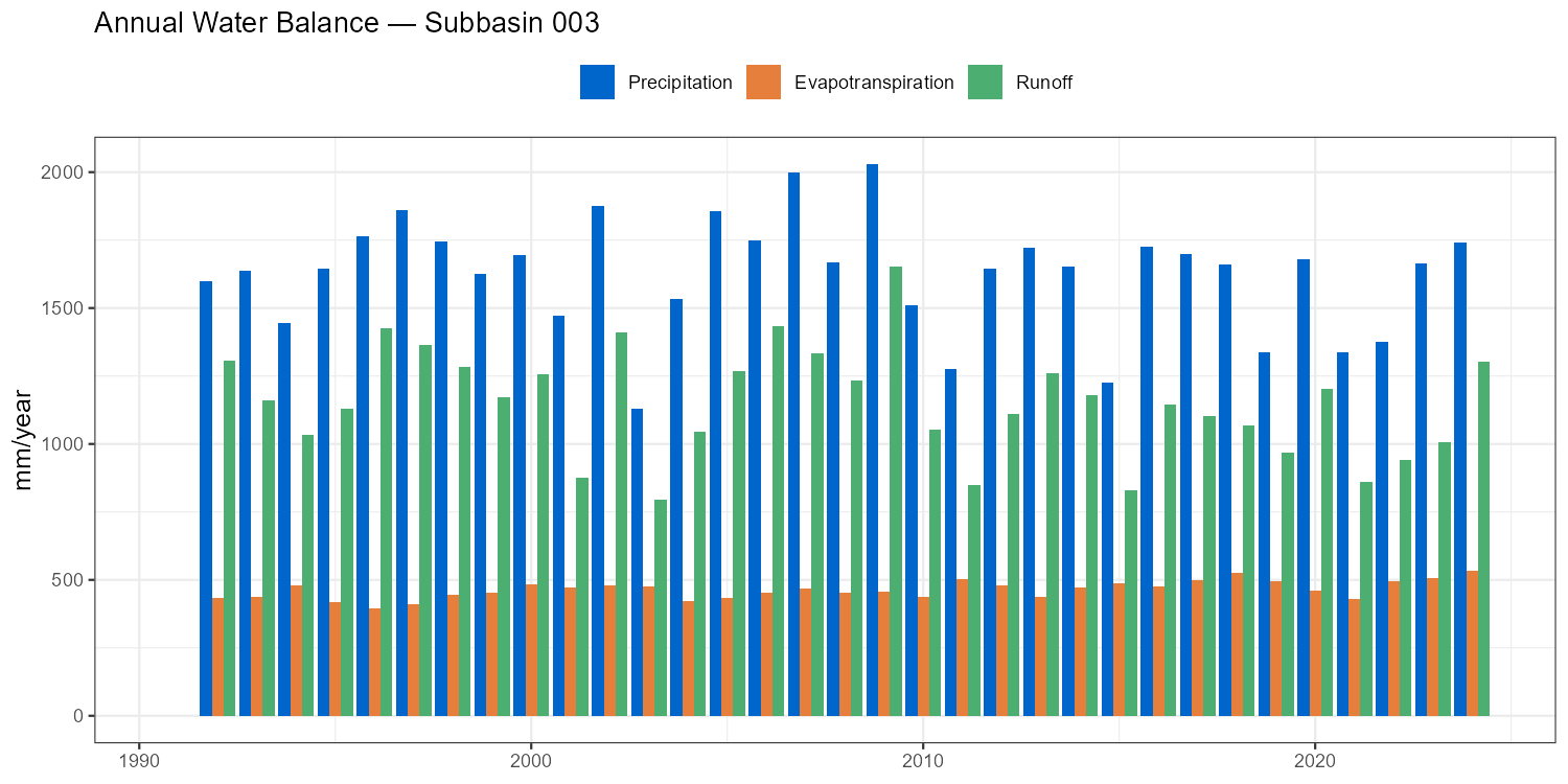
Monthly Water Balance Components
Show/hide: Monthly water balance
# Double group_by: first sum daily → monthly totals per year, then average across years
monthly_clim <- wb |>
  mutate(
    Date  = as.Date(DateTime),
    Year  = as.integer(format(Date, "%Y")),
    Month = as.integer(format(Date, "%m"))
  ) |>
  group_by(Year, Month) |>
  summarise(
    P    = sum(.data[[paste0("PGEB_",   sb_id)]], na.rm = TRUE),
    ETAT = sum(.data[[paste0("ETAGEB_", sb_id)]], na.rm = TRUE),
    Q    = sum(.data[[paste0("QABGEB_", sb_id)]], na.rm = TRUE),
    .groups = "drop"
  ) |>
  group_by(Month) |>
  summarise(P = mean(P), ETAT = mean(ETAT), Q = mean(Q), .groups = "drop")

p_mon_wb <- ggplot(monthly_clim, aes(x = Month)) +
  geom_col(aes(y = P, fill = "Precipitation"), alpha = 0.5, width = 0.7) +
  geom_line(aes(y = Q,    colour = "Runoff"),    linewidth = 1.1) +
  geom_line(aes(y = ETAT, colour = "Actual ET"), linewidth = 1.1, linetype = "dashed") +
  geom_point(aes(y = Q,    colour = "Runoff"),    size = 2) +
  geom_point(aes(y = ETAT, colour = "Actual ET"), size = 2, shape = 21, fill = "white") +
  scale_x_continuous(breaks = 1:12, labels = month.abb) +
  scale_fill_manual(  values = c("Precipitation" = "#AED6F1")) +
  scale_colour_manual(values = c("Runoff" = "#5E4B8B", "Actual ET" = "#E67E3C")) +
  labs(title = paste("Mean Monthly Water Balance — Subbasin", target_subbasin),
       x = NULL, y = "mm/month", fill = NULL, colour = NULL) +
  theme_bw() + theme(legend.position = "top",
                     axis.title = element_text(size = 12))
print(p_mon_wb)
ggsave(file.path(plot_dir, paste0("monthly_wb_NB", target_subbasin, ".png")),
       p_mon_wb, width = 8, height = 5, dpi = 150)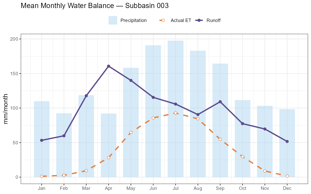
NoteWhat to check in the water balance
- Runoff ratio Q/P: Alpine catchments typically 0.50–0.80. Values above 1.0 indicate a structural error.
- Actual ET: Should be 200–600 mm/year in the Austrian Alps. Implausibly low values suggest PCOR is inflating precipitation to compensate for poor calibration.
Part 8: Spatial Outputs
NoteWhat you’ll learn
Link COSERO output to the GIS zones shapefile and produce spatial maps of calibrated parameters. Spatial patterns should be physically interpretable — if a parameter map shows no spatial variation, that is itself diagnostic information. Displaying spatial patterns of runoff components or evapotranspiration is also possible, but requires to run COSERO with OUTPUTTYPE = 3 and OUTCONTROL = 1.
Reading the Zones Shapefile
# Path to zones shapefile — created in Module 2 (adjust filename to your project)
zones_shp  <- st_read(file.path(project_path, "GIS/Shapefiles/wildalpen_cosero_zones.shp"),
                       quiet = TRUE)

cat(sprintf("Zones: %d  |  Subbasins: %s\n",
            nrow(zones_shp),
            paste(sort(unique(zones_shp$NB)), collapse = ", ")))

# Read calibrated parameter file (all columns, one row per zone)
params_cal <- read_cosero_parameters(par_file_cal)

# Merge parameters onto the spatial data frame
zones_cal  <- merge(zones_shp, params_cal, by.x = "NZ", by.y = "NZ_",
                    all.x = TRUE)
Parameter Maps
Show/hide: Parameter map grid
# Compute annual mean PCOR from monthly columns (PCor1_ … PCor12_)
pcor_cols    <- paste0("PCor", 1:12, "_")
pcor_present <- pcor_cols[pcor_cols %in% colnames(zones_cal)]
if (length(pcor_present) > 0)
  zones_cal$PCOR_mean <- rowMeans(st_drop_geometry(zones_cal)[, pcor_present, drop = FALSE],
                                  na.rm = TRUE)

# Select parameters to map — include PCOR_mean if available
map_params <- c("M_", "BETA_", "KBF_", "TAB1_", "CTMAX_",
                if ("PCOR_mean" %in% colnames(zones_cal)) "PCOR_mean")

plots_map <- lapply(map_params, function(par) {
  if (!par %in% colnames(zones_cal)) return(NULL)
  label <- gsub("_mean$", "", gsub("_$", "", par))   # strip trailing _ or _mean suffix
  ggplot(zones_cal) +
    geom_sf(aes(fill = .data[[par]]), colour = NA) +
    scale_fill_viridis_c(option = "D", name = label) +
    labs(title = label) +
    theme_void() +
    theme(plot.title = element_text(face = "bold", size = 11))
})
plots_map <- Filter(Negate(is.null), plots_map)

wrap_plots(plots_map, ncol = 3) +
  plot_annotation(title    = "Calibrated Parameter Maps",
                  subtitle = "One value per COSERO zone")

ggsave(file.path(plot_dir, "parameter_maps_calibrated.png"),
       width = 15, height = 10, dpi = 150)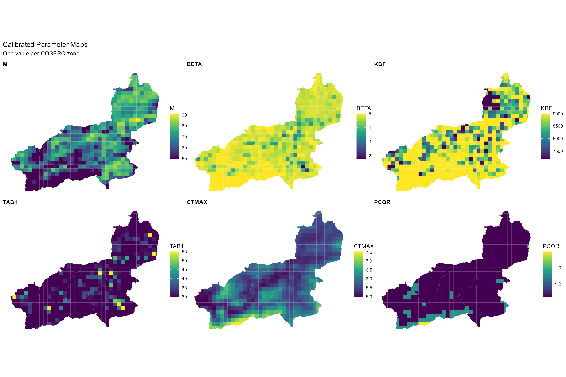
Elevation-Dependent Patterns
Parameters, e.g. related to snow and temperature, typically show a clear elevation gradient. Checking whether the calibrated values preserve this gradient is a good physical plausibility test.
Show/hide: Elevation vs. CTMAX scatter
# Requires ELEV_ attribute in the shapefile (added during Module 2 zone generation)
if (all(c("CTMAX_", "ELEV_") %in% colnames(zones_cal))) {
  p_ctmax <- ggplot(zones_cal, aes(x = ELEV_, y = CTMAX_)) +
    geom_point(alpha = 0.5, size = 1.5, colour = "#5E4B8B") +
    geom_smooth(method = "loess", colour = "#E67E3C", se = TRUE) +
    labs(title    = "Snowmelt Factor (CTMAX) vs. Mean Zone Elevation",
         x = "Mean elevation (m a.s.l.)", y = "CTMAX (mm/°C/day)") +
    theme_bw() + theme(axis.title = element_text(size = 12))
  print(p_ctmax)
  ggsave(file.path(plot_dir, "ctmax_vs_elevation.png"),
         p_ctmax, width = 7, height = 5, dpi = 150)
}
Part 9: Synthesis & Evaluation Checklist
Use the checklist below as a structured self-assessment before your group presentation. Every row corresponds to something you should be able to answer or show a figure for.
| Aspect | Question to answer | Where to look |
|---|---|---|
| Overall performance | Are NSE and KGE acceptable for both cal and val? | Part 5 |
| Volume bias | Is BETA close to 1.0 in both periods? | Part 5 |
| Validation drop | How large is the performance drop in validation? | Part 5 |
| Peak flows | Are flood peaks reproduced in timing and magnitude? | Part 6 — events |
| Low flows | Does the model reproduce the baseflow recession? | Part 6 — FDC |
| Residual patterns | Any seasonal or long-term systematic bias in residuals? | Part 6 |
| Seasonal regime | Does the monthly regime match the observed timing? | Part 6 |
| Water balance | Is the annual residual (P − ET − Q − ΔS) small in most years? Are the annual ET and Q totals in a physically plausible range? | Part 7 |
| Runoff composition | Which pathway dominates — surface, interflow, or baseflow? Is this consistent with the catchment’s geology and land use? | Part 7 |
| Internal states | Is snow cover seasonal, soil moisture seasonal, groundwater stable? | Part 7 |
| Spatial patterns | Do parameter maps show physically meaningful spatial variability? | Part 8 |
| Limitations | Can you name at least two concrete model limitations? | Below |
ImportantThe model is a simplification — report this honestly
No hydrological model is “correct”. A high calibration NSE means the optimiser found parameter values that minimise the chosen error metric over the calibration period. It does not prove that the model correctly represents internal processes, that the parameters are physically meaningful, or that the model will perform well under changed conditions. In your presentation, always report:
- Which parameters were calibrated and which were kept at defaults
- The objective function(s) and algorithm used
- Performance for both calibration and validation periods
- At least two known model limitations
Common COSERO model limitations to consider:
- Precipitation uncertainty: SPARTACUS grid interpolation may smooth out local convective events; orographic enhancement in small high-alpine sub-catchments may be underrepresented; station coverage may be limited.
- No explicit karst or deep groundwater: Subsurface losses to karst systems or interbasin groundwater transfers are not represented — a systematic dry bias in spring-dominated catchments is a likely symptom.
- Equifinality: Many parameter combinations can produce a similar NSE. The calibrated set is one behavioural solution, not the physically correct one.
- Parameter stationarity: Calibrated parameters are assumed constant in time. Land use change, vegetation dynamics, or non-stationarity in precipitation–runoff relationships are not captured.
- A priori parameter uncertainty: Initial parameter fields are derived from Austria-wide raster datasets at 1 km resolution (see Module 2 — Parameter Raster Downloads). These rasters carry their own methodological, mapping and spatial aggregation errors, which propagate into the calibration starting point and constrain the solution space.
What You Should Know
After completing this module you should be able to apply and explain all of the following steps for your own catchment.
Calibration and validation concepts. Explain the split-sample test and its purpose. Define equifinality and explain why a high NSE does not imply a correct model. Name two things calibration cannot fix (e.g. wrong input data, missing processes, scale mismatches; see Equifinality and the Limits of Calibration in Part 1).
Parameter selection and bounds. Justify which parameters you selected for calibration, referencing the Sobol total-effect indices from Module 3. Explain how narrowing bounds based on behavioural ranges can improve calibration efficiency without losing physical plausibility.
DDS calibration. Explain the DDS algorithm’s core principle (progressively reducing the probability of perturbing each dimension as iterations increase). Run a calibration, interpret the convergence plot, and compare initial versus calibrated performance for each subbasin. Know when to consider SCE-UA as an alternative.
Split-sample validation. Report NSE, KGE, and BETA for both periods. Diagnose the cause of any performance drop in validation and articulate what it implies about model transferability.
Hydrograph diagnostics. Identify systematic residual patterns (seasonal bias, peak underestimation, baseflow overestimation) and link them to specific model processes or parameters. Zoom into at least two contrasting events and describe their performance differences.
Water balance. Inspect the annual water balance table: are the residuals (P − ET − Q − ΔS) small relative to P? Are the annual ET and Q totals credible given the catchment’s climate and elevation? Describe what each of the three runoff components (surface runoff, interflow, baseflow) represents and which pathway dominates in your catchment.
Spatial patterns. Produce at least two calibrated parameter maps and discuss the spatial variability. Verify that elevation-dependent parameters (e.g. CTMAX, PCOR) follow a physically plausible gradient.
Critical synthesis. Identify the main limitations of your model and propose at least one concrete improvement — a different process representation, a changed parameter bound, or a data quality fix. Your grade is not determined by your NSE score but by the quality of your critical interpretation.
Document created: 2026-05-22
References
Beven, K. J.: Rainfall-runoff modelling: The primer, John Wiley & Sons, Chichester, 2001.
Duan, Q., Gupta, V. K., and Sorooshian, S.: Shuffled complex evolution approach for effective and efficient global minimization, Journal of Optimization Theory and Applications, 76, 501–521, https://doi.org/10.1007/BF00939380, 1993.
Gupta, H. V.: Deep learning can facilitate physically interpretable geoscientific modelling, Nature Water, 4, 118–119, https://doi.org/10.1038/s44221-026-00589-x, 2026.
Kirchner, J. W.: Getting the right answers for the right reasons: Linking measurements, analyses, and models to advance the science of hydrology, Water Resources Research, 42, W03S04, https://doi.org/10.1029/2005WR004362, 2006.
Klemeš, V.: Dilettantism in hydrology: Transition or destiny?, Water Resources Research, 22, S177–S188, https://doi.org/10.1029/WR022i09Sp0177S, 1986.
Tolson, B. A. and Shoemaker, C. A.: Dynamically dimensioned search algorithm for computationally efficient watershed model calibration, Water Resources Research, 43, W01413, https://doi.org/10.1029/2005WR004723, 2007.