library(CoseRo)

# Creates a ready-to-run example project (Wildalpen catchment)
setup_cosero_project_example("C:/COSERO/Wildalpen_example")

# Optionally run it straight away
run_cosero("C:/COSERO/Wildalpen_example")Mathew Herrnegger · mathew.herrnegger@boku.ac.at
Institute of Hydrology and Water Management (HyWa) BOKU University Vienna, Austria
LAWI301236 · Distributed Hydrological Modeling with COSERO
![]()
Introduction
This module covers the spatial setup of your COSERO model and the processing of meteorological input data from SPARTACUS. You will work with QGIS and R to prepare the spatial structure and extract gridded climate data.
Learning Objectives:
- Understand COSERO’s state-space formulation and spatial discretization
- Work with Hydrological Atlas catchment polygons in QGIS
- Aggregate catchments to appropriate spatial scales
- Read and process SPARTACUS NetCDF files in R
- Generate COSERO input files
Setting Up the Project Directory
Before starting any practical work, you need a well-organised working directory. COSERO requires a specific folder structure with separate input and output subfolders alongside the model executable. The CoseRo package provides two helper functions to create this structure automatically.
Option A — Example project: Creates a fully working project pre-populated with the Wildalpen example catchment, including COSERO binaries, all input files, and example outputs. Use this to test the setup or as a template and substitute the inputs with the files you generate.
Option B — Empty project (for your own catchment): Creates the folder structure and copies the COSERO binaries, but leaves all input files for you to fill in.
library(CoseRo)

# Creates an empty project structure for your own catchment
setup_cosero_project(
  project_path    = "C:/COSERO/MyCatchment",
  create_defaults = TRUE
)
A typical COSERO project directory looks like this:
D:/COSERO/Wildalpen/
├── COSERO.exe                    ← model executable
├── libiomp5md.dll                ← required runtime library
├── libiomp5md.lib
├── cosero_commands.txt           ← command-line arguments passed to COSERO.exe
├── run_cosero_temp.bat           ← temporary batch file generated by run_cosero()
├── input/
│   ├── defaults.txt              ← global model settings (simulation period, spinup, output type)
│   ├── MetDefaults.txt           ← meteorological input file references
│   ├── para_ini.txt              ← zone parameters
│   ├── parameterfile_backup/     ← automatic backups of parameter files (created by CoseRo)
│   ├── P_NZ_1991_2024.txt        ← precipitation input (zonal, plain text)
│   ├── P_NZ_1991_2024.bin        ← precipitation input (binary, faster I/O)
│   ├── T_NZ_1991_2024.txt        ← temperature input
│   ├── T_NZ_1991_2024.bin
│   ├── Qobs.txt                  ← observed discharge for calibration/validation
│   ├── Qadd_example.txt          ← example file for additional discharge inputs
│   ├── reg_para_example.txt      ← example regression settings file
│   ├── radmat.par                ← radiation parameters for glacier module
│   └── raster_write.txt          ← spatial output configuration
└── output/                       ← model outputs written here after each run
    ├── COSERO.runoff             ← simulated discharge
    ├── COSERO.prec               ← precipitation
    ├── COSERO.plus               ← runoff components
    ├── COSERO.plus1              ← water balance states
    ├── parameters.txt            ← parameter echo (copy of para_ini.txt used in run)
    ├── statistics.txt            ← performance metrics (NSE, KGE, BETA, ...)
    ├── topology.txt              ← subbasin routing topology
    ├── statevar.dmp              ← saved model state (for warm start)
    └── ...                       ← depending on settings in defaults.txt, different additional files are written to output
This structure was created with setup_cosero_project_example("D:/COSERO/Wildalpen") and is used as the demonstration project throughout this course.
Tip
Adapt the project path to your system. On Windows, avoid paths with spaces or special characters (e.g., use C:/COSERO/ rather than C:/My Documents/).
Case Study: Salza River at Wildalpen
Throughout this course, we demonstrate the complete COSERO model setup using the Salza catchment in the Hochschwab region of Styria, Austria.
- Location: Northern Limestone Alps, Upper Styria, draining to the Enns River
- Catchment area: ~592 km² at the Wildalpen gauge
- Characteristics: Steep terrain, pronounced karst hydrology, strong snow and snowmelt influence, nival-pluvial discharge regime
- Data availability: Multiple eHYD gauging stations with long records, full SPARTACUS coverage
The Hochschwab Massif and Vienna’s Water Supply
The Hochschwab Massif is not merely an interesting alpine catchment for hydrological teaching — it is the primary source of drinking water for the city of Vienna. The Second Vienna Spring Pipeline (II. Hochquellenleitung, II. HQL; constructed 1900–1910) draws its water from springs in the Hochschwab karst system and delivers it to Vienna over approximately 183 km entirely by gravity — no pumping is required under normal operation, making the system energetically self-sufficient and highly reliable (Gemeinderatsausschuß der Stadt Wien, 1910). The hydraulic pressure along the pipeline is additionally used to generate electricity at several in-line hydropower stations (e.g. Gaming). From source to the Lainz reservoir in Vienna, the water travels for approximately 36 hours (Zweite Hochquellenleitung, 2025).
In the long-term annual mean, the II. HQL supplies approximately 53 % of Vienna’s total drinking water demand, making it the city’s single largest supply source. The I. HQL (from the Rax–Schneeberg area) contributes around 43 %, with the remaining 4 % covered by groundwater works (Donauinsel, Lobau, Moosbrunn) which serve primarily as peak-demand reserves and emergency backup (Koblizek and Süssenbek, 1999--2000; Wiener Wasser: Zahlen, Daten, Fakten, 2025). Strict source protection in the catchment ensures water quality that typically requires no chemical treatment (Stadt Wien - Wiener Wasser, 2023).
The central spring of the system is the Kläfferquelle in the Salzatal (Koppensteiner and Plan, 2019; Plan et al., 2010) — one of the most productive drinking water springs in Europe. As a classic Alpine limestone karst spring, its discharge is tightly coupled to current precipitation and snowmelt conditions: winter low flows can fall below 400 l/s, while peak discharges during summer thunderstorms or spring snowmelt can exceed 45,000 l/s (August 2006), with a long-term mean discharge of approximately 5,150 l/s (1995–2006). The seasonal regime is dominated by snowmelt processes, with highest monthly mean discharges occurring between May and August and lowest values in winter. The karst system’s limited storage capacity means the spring responds rapidly to meteorological forcing, and turbidity events — caused by heavy thunderstorms in summer or by increased shearing forces in karst conduits during snowmelt — are a characteristic feature of the spring dynamics.
Delineating the catchment area of the Kläfferquelle is inherently difficult. Geological mapping and structural geology analyses suggest a maximum catchment size of 60–70 km², centred on the Hochschwab plateau. However, hydrological delineation is complicated by the absence of precipitation stations on the plateau, limited discharge measurement infrastructure at the springs, and the possibility of shifting catchment boundaries under different hydrological conditions — a common challenge in karstic systems. Oxygen-18 isotope fractionation analyses indicate a mean catchment altitude of approximately 1,700 m a.s.l., consistent with morphometric and geological mapping results. Continuous hydrological monitoring — and, by extension, distributed hydrological modelling — is therefore essential for understanding and managing long-term water availability under a changing climate (Plan et al., 2010).
ImportantKarst Uncertainty: Orographic ≠ Hydrological Catchment
In karst systems such as the Hochschwab, orographic catchment boundaries derived from a DEM do not necessarily coincide with the true hydrological catchment. Precipitation falling within the topographic divide may be routed underground through conduit networks and fractures to springs outside the orographic boundary — and vice versa. Catchment boundaries can also shift depending on hydrological conditions. The Kläfferquelle’s actual recharge area is therefore not fully captured and is unknown.
This introduces a fundamental uncertainty in any rainfall-runoff model applied here: the effective contributing area is unknown, precipitation inputs may be systematically over- or underestimated, and water balance closure cannot be guaranteed from surface data alone. The Hochschwab is therefore a good example of a broader challenge in karst hydrology — even before a single parameter is estimated or a simulation is run, the definition of the system itself carries substantial uncertainty.
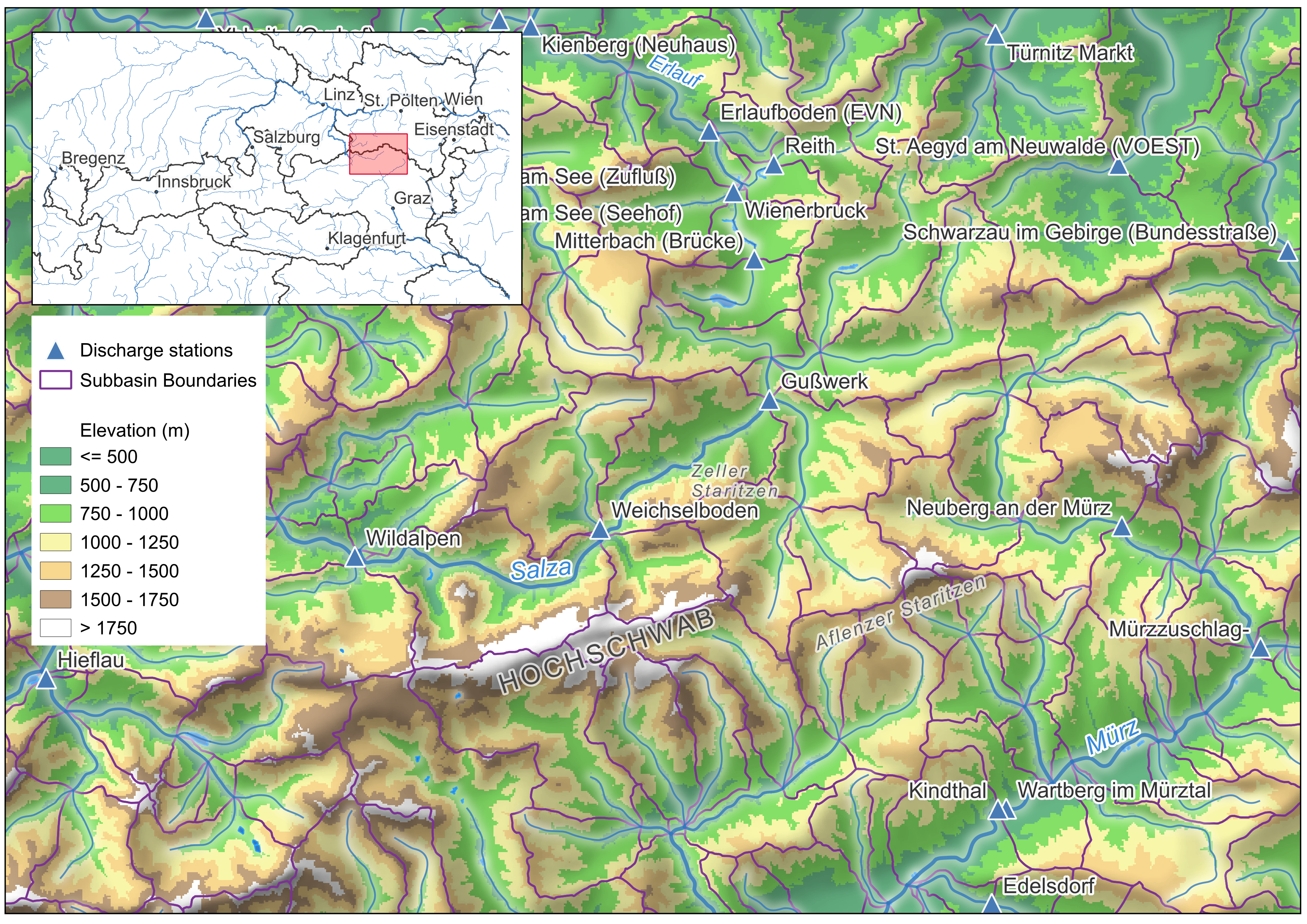
The map shows the spatial data you will work with:
- Purple lines: Sub-catchment boundaries from eHAO (Hydrological Atlas of Austria)
- Blue lines: River network (eHAO)
- Blue triangles: Gauging station locations (eHAO) — discharge time series are downloadable from eHYD
ImportantSelect Your Own Catchment
Part 1: Spatial Setup — Delineation, Zones & Initial Parameters
Downloading Data from eHAO
The eHAO (Hydrologischer Atlas Österreichs) is the primary source for spatial data needed to set up a COSERO model in Austria. It provides catchment boundary polygons, river networks, gauging stations, and many thematic layers. The portal is operated by BOKU together with the Austrian Federal Ministry.
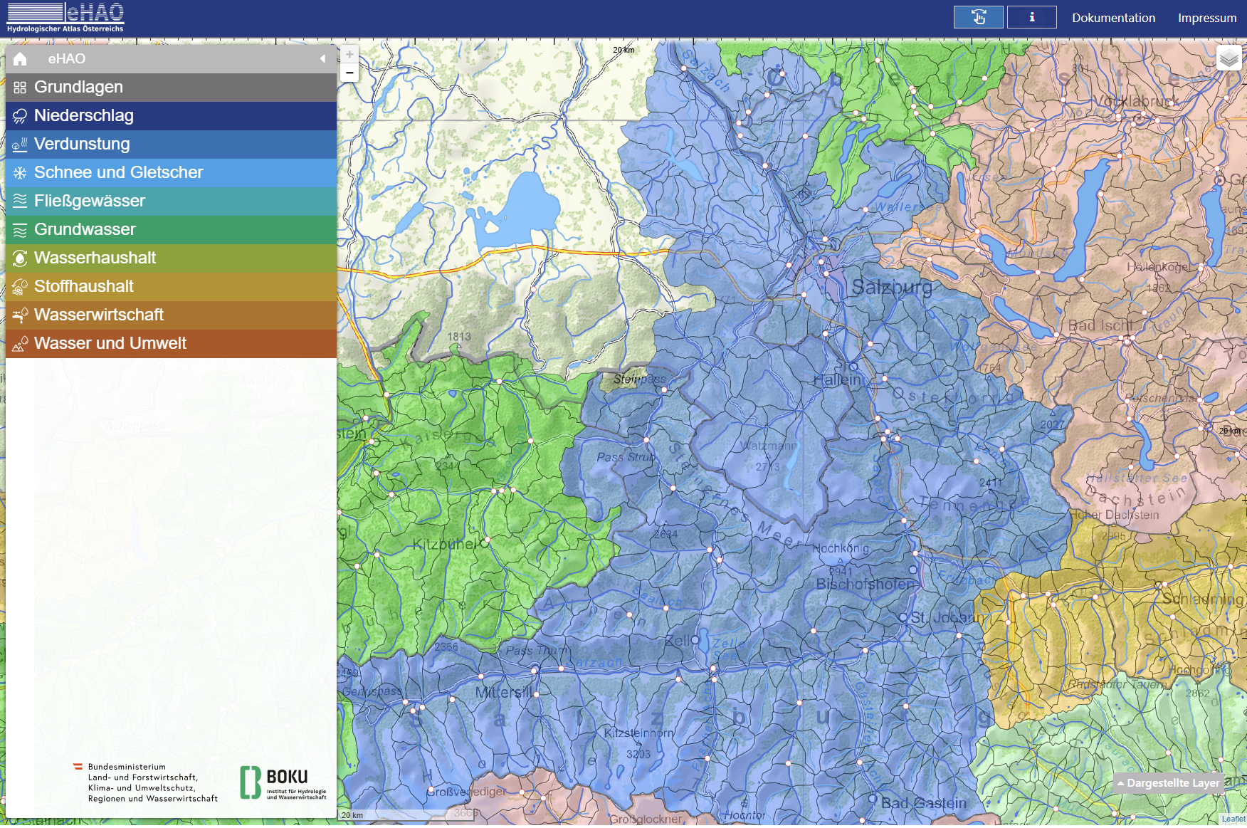
Download the following three datasets:
| Layer | eHAO section | What to download |
|---|---|---|
| Catchment boundaries | 1. Grundlagen → 1.3 Einzugsgebietsgliederung | Einzugsgebiete (polygons) |
| River network | 1. Grundlagen → 1.2 Fließgewässer und Seen | Fließgewässer (lines) |
| Gauging stations | 5. Fließgewässer & Seen → 5.1 → Alle Pegel | Durchfluss (points) |
For example, the catchment boundaries can be downloaded from the Einzugsgebiete layer under section 1.3 by clicking the download button (circled in red below):
Proceed in a similar manor for the other layers.
NoteGIS Data Downloads
As an alternative, the spatial datasets needed for this module are provided below. Download the files and save them to a known location on your computer (e.g. C:/COSERO/GIS/).
| File | Description | Source |
|---|---|---|
| COP90m_DEM_31287.tif | Copernicus 90 m DEM, Austria, EPSG:31287 | European Space Agency (2024) |
| gemeinsam_gew1mio.zip | River network | eHAO |
| k1_3_wasserbilanz.zip | Catchment boundaries (Wasserbilanz) | eHAO |
| k5_1_gpegel.zip | Gauging stations | eHAO |
| SPARTACUS_grid_31287.zip | SPARTACUS 1 km grid polygons, EPSG:31287 | Generated from GeoSphere Austria NetCDF — see Step 2 |
Shapefiles are provided as zip archives containing all component files (.shp, .dbf, .prj, .shx). Extract to your GIS folder before loading in QGIS.
Visualising Your Catchment in QGIS
Before delineating or merging subbasins, it is important to explore the data visually and connect the abstract geodata with the real landscape. A well-composed map helps you understand the topography, identify where rivers flow, and decide how to group sub-catchments into subbasins. You can also add satellite imagery or other basemaps using the plugin “Quickmapservices” for better orientation and understanding the landscape.
Load all layers into QGIS:
- Open QGIS and create a new project (Project → New).
- Add all downloaded files using the
Data Source Manager(CTRL+L). - If no CRS (Coordinate Reference System) is detected in QGIS, define
EPSG:31287by clicking on the button on lower right corner of the QGIS window.
Style the layers to make the map readable:
- Catchment polygons — set fill to transparent and give the border a clear colour (e.g. dark blue). Right-click the layer → Properties → Symbology → Simple Fill → Fill style: No Brush.
- River network — use a blue line, adjust width to 0.2–0.6 mm.
- Gauging stations — use a distinct marker (e.g. triangle or circle). Add labels showing the station name or ID: right-click → Properties → Labels → Single Labels, and select the appropriate attribute (e.g.
name) from the attribute table. Open the attribute table (right-click → Open Attribute Table) to inspect available fields first. In the attribute table you will also find thehzbnr, which is the ID used by the National Hydrographic Service of Austria. - DEM hillshade — to show topography, duplicate the DEM layer and set one copy to Symbology → Hillshade (illumination from the north-west). Place it beneath all vector layers and set transparency to ~50%. This immediately reveals valleys, ridges, and how the river network connects to the terrain.
TipWhy bother with symbology?
These are not just technical layers — they represent a real landscape with mountains, valleys, rivers, and measurement stations. A well-styled map makes it immediately clear where a catchment lies, which tributaries feed it, and where discharge is measured. This visual understanding is essential before making any modelling decisions.
ImportantCheck your data
Once layers are loaded, use the Identify Features tool to click on polygons and points and inspect their attribute values. Verify that the gauging station IDs and catchment identifiers are consistent — you will need them when assigning NB values and matching discharge observations.
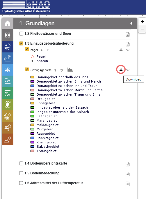
Step 1: Subbasin Delineation in QGIS
The first step is to define the subbasins (NB) — the major spatial units for which COSERO simulates discharge. Subbasin boundaries are derived from the small pre-delineated sub-catchments provided by the eHAO (Hydrological Atlas of Austria). These fine-scale units are merged in QGIS using gauging stations as outlets, so that each resulting subbasin drains to exactly one gauging station.
Each subbasin is assigned a unique integer identifier (NB) in upstream-to-downstream order: headwater subbasins receive the lowest NB values, and the most downstream subbasin the highest. This ordering is required by COSERO for correct flow routing.
The goal of this step is to produce a subbasin shapefile like the one shown below for the Salza/Wildalpen example — three subbasins numbered 1 (most upstream, Gußwerk) through 3 (most downstream, Wildalpen):
Workflow in QGIS:
1. Select and export the relevant gauges
From the full Austria-wide gauging station layer (k5_1_gpegel), select only the gauges within your modelling area using Select Features by Area or Single Click (hold Shift to add to the selection). Then right-click the layer → Export → Save Selected Features As… and save as e.g. cosero_gauges.shp. Add this new layer to the map and switch off the original Austria-wide layer to avoid confusion.
2. Select and export the relevant sub-catchments
Do the same for the catchment boundaries layer (k1_3_wasserbilanz): select all sub-catchments that fall within your study area, right-click → Export → Save Selected Features As… and save as e.g. cosero_subbasins.shp. Style the new layer (transparent fill, coloured border) and switch off the original.
3. Merge sub-catchments into subbasins
Working on the cosero_subbasins layer:
- Enable editing: click the Toggle Editing pencil icon in the toolbar (or right-click layer → Toggle Editing).
- Use Select Features by Area or Single Click (hold Shift to multi-select) to select all sub-catchments that belong to the first subbasin (e.g. all polygons draining to gauge NB = 1).
- Go to Edit → Merge Selected Features. In the dialog, choose Take attributes from the largest geometry (or set values manually). Confirm with OK.
- Repeat for each remaining subbasin.
- Save edits by clicking the Toggle Editing pencil again and confirming Save.
4. Add and populate the NB field
- Open the attribute table (right-click layer → Open Attribute Table).
- Click Add Field (pencil + icon), name it
NB, type Integer. - For each merged polygon, enter the NB value: NB = 1 for the most upstream subbasin, incrementing downstream. Click into the cell to edit directly (editing mode must be active).
- Save edits by toggling the pencil off.
ImportantNB ordering matters
COSERO’s routing algorithm requires subbasins to be numbered strictly upstream to downstream: NB = 1 is the headwater subbasin farthest from the outlet, and the highest NB is the most downstream subbasin (main catchment outlet). Incorrect ordering will produce wrong routing results.
The resulting shapefile must contain at minimum the field NB (integer subbasin ID).
TipCatchment and Stream Network Delineation in QGIS
If your catchment boundaries are not yet available from eHAO, or you wish to delineate subbasins from scratch using a DEM (e.g. for a catchment in a different part of the world), QGIS supports a full workflow for automated catchment and stream network delineation. The key steps are DEM conditioning (pit-filling, breach processing), flow direction and accumulation, channel network extraction, and watershed delineation from pour points.
WhiteboxTools is the recommended toolset for this workflow. It provides robust, hydrologically-aware DEM processing algorithms — particularly its breach and depression-filling routines — that outperform the equivalent SAGA and GDAL tools for complex terrain. WhiteboxTools integrates directly into QGIS via the WhiteboxTools for QGIS plugin (install via Plugins → Manage and Install Plugins) and can also be called from R using the whitebox package.
Lecture notes covering this workflow in detail are available here:
Step 2: Generating the SPARTACUS Grid Shapefile
Downloading a SPARTACUS NetCDF File
The grid shapefile is derived from the coordinate information embedded in a SPARTACUS NetCDF file. At this stage you only need a single file — it is used exclusively to extract the grid geometry, not for meteorological modelling yet. Download the 1961 precipitation file (≈ 14 MB):
SPARTACUS2-DAILY_RR_1961.nc Source: GeoSphere Austria Data Hub — SPARTACUS v2.1 daily 1 km
Save this file to a known location, for example C:/COSERO/data/SPARTACUS2-DAILY_RR_1961.nc, and update the nc_file path in the script below accordingly.
Generating the Grid Shapefile
In our example, COSERO zones are defined by intersecting the subbasin boundaries with a spatial grid. For Austrian catchments, the natural choice is the SPARTACUS 1 km × 1 km grid (EPSG: 31287), which directly corresponds to the meteorological input data. The grid shapefile is generated from the SPARTACUS NetCDF file using the R script:
This script reads the projected x/y coordinates from the NetCDF file and constructs 1 km² polygon cells, numbered from upper-left (NW) to lower-right (SE). The output is a polygon shapefile that serves as the spatial template for zone generation.
Show/hide: create_spartacus_grid_shapefile.R
################################################################################
# Create SPARTACUS Grid Shapefile from NetCDF
# Creates polygon shapefile with ID (upper-left to lower-right), row, col attributes
# Grid is in EPSG:3416 (ETRS89 / Austria Lambert), 1km resolution
################################################################################

library(ncdf4)
library(sf)
library(terra)

#===============================================================================
# USER SETTINGS — adapt these paths to your system
#===============================================================================

# Path to a single downloaded SPARTACUS NetCDF file (any year, RR variable)
# Download from: https://public.hub.geosphere.at/datahub/resources/spartacus-v2-1d-1km/
nc_file <- "C:/COSERO/MyCatchment/data/SPARTACUS2-DAILY_RR_1961.nc"

# Output directory — grid shapefiles and reference GeoTIFF will be written here
output_dir <- "C:/COSERO/MyCatchment/GIS/SPARTACUS_grid/"

#===============================================================================
# DERIVED OUTPUT PATHS — no changes needed below this line
#===============================================================================

output_shp     <- file.path(output_dir, "SPARTACUS_grid_3416.shp")
output_tif     <- file.path(output_dir, "SPARTACUS_RR_1961_day1_3416.tif")
output_shp_31287 <- file.path(output_dir, "SPARTACUS_grid_31287.shp")
output_tif_31287 <- file.path(output_dir, "SPARTACUS_RR_1961_day1_31287.tif")

# Create output folder if it doesn't exist
if (!dir.exists(output_dir)) {
  dir.create(output_dir, recursive = TRUE)
  cat(sprintf("Created folder: %s\n", output_dir))
}

# Open NetCDF and extract x/y coordinates (projected, cell centers)
nc <- nc_open(nc_file)
x <- nc$dim$x$vals  # 584 values, west to east
y <- nc$dim$y$vals  # 329 values, south to north (increasing)
nc_close(nc)

# Grid dimensions
n_col <- length(x)  # 584
n_row <- length(y)  # 329
cat(sprintf("Grid: %d cols x %d rows = %d cells\n", n_col, n_row, n_col * n_row))

# Cell half-size (1km grid)
d <- 500  # meters

# Reverse y so row 1 = north (top), row 329 = south (bottom)
y_rev <- rev(y)

# Create polygons: ID=1 at upper-left (NW), max at lower-right (SE)
polygons <- vector("list", n_col * n_row)
id <- 1

for (r in 1:n_row) {
  y_center <- y_rev[r]
  for (c in 1:n_col) {
    x_center <- x[c]

    # Polygon corners (counter-clockwise for sf)
    coords <- matrix(c(
      x_center - d, y_center - d,
      x_center + d, y_center - d,
      x_center + d, y_center + d,
      x_center - d, y_center + d,
      x_center - d, y_center - d
    ), ncol = 2, byrow = TRUE)

    polygons[[id]] <- st_polygon(list(coords))
    id <- id + 1
  }
}

# Build sf object
geom <- st_sfc(polygons, crs = 3416)
grid_sf <- st_sf(
  ID  = 1:(n_col * n_row),
  row = rep(1:n_row, each = n_col),
  col = rep(1:n_col, times = n_row),
  geometry = geom
)

# Write shapefile
st_write(grid_sf, output_shp, delete_layer = TRUE)
cat(sprintf("Written: %s\n", output_shp))
cat(sprintf("ID: 1 (upper-left/NW) to %d (lower-right/SE)\n", n_col * n_row))

# Save first time step as GeoTIFF for cross-checking
# Force values to be computed (applies scale_factor from NetCDF)
r <- rast(nc_file, subds = "RR")[[1]]  # first day
values(r) <- values(r)  # materialize scaled values
writeRaster(r, output_tif, overwrite = TRUE)
cat(sprintf("Written: %s\n", output_tif))

# Transform and save in EPSG:31287 (MGI / Austria Lambert)
grid_sf_31287 <- st_transform(grid_sf, 31287)
st_write(grid_sf_31287, output_shp_31287, delete_layer = TRUE)
cat(sprintf("Written: %s\n", output_shp_31287))

# Use same CRS string from sf to ensure consistent datum transformation
# method="near" preserves original values (no interpolation)
crs_31287 <- st_crs(grid_sf_31287)$wkt
r_31287 <- project(r, crs_31287, method = "near")
writeRaster(r_31287, output_tif_31287, overwrite = TRUE)
cat(sprintf("Written: %s\n", output_tif_31287))

# Check values didn't change
cat(sprintf("Original range: %.2f - %.2f\n", minmax(r)[1], minmax(r)[2]))
cat(sprintf("Reprojected range: %.2f - %.2f\n", minmax(r_31287)[1], minmax(r_31287)[2]))
NoteAlternative: Classical HRUs
Instead of intersecting with the meteorological grid, zones can also be defined as classical Hydrological Response Units (HRUs) by overlaying subbasin polygons with land use maps, elevation zones, and/or soil type maps. This approach groups physically similar areas within a subbasin regardless of the grid geometry.
Step 3: Generating COSERO Zones, IDs, and Routing
Once the subbasin shapefile and the grid are available, the full zone structure — including zone IDs, elevation statistics, and the routing network — is generated automatically using:
Show/hide: generate_cosero_zones.R
################################################################################
# Generate COSERO zones from subbasins and SPARTACUS grid
#
# Workflow:
#   1. Intersect subbasins with grid
#   2. Remove small zones (<0.25 km²) by merging within subbasin
#   3. Assign NZ/IZ based on elevation, outlet zone near gauge
#   4. Calculate ToNZ routing and downstream distances
#
# Requirements:
#   - R packages: sf, terra, dplyr, exactextractr, ggplot2, patchwork
#   - install.packages(c("sf", "terra", "dplyr", "exactextractr", "ggplot2", "patchwork"))
#
# Input files:
#   - subbasins_shp: Polygon shapefile with field "NB" (subbasin ID, integer)
#   - grid_shp:      SPARTACUS grid polygons (from create_spartacus_grid_shapefile.R)
#   - dem_tif:       DEM raster for elevation calculation
#   - gauges_shp:    Point shapefile with field "NB" (matching subbasin ID)
#
# Output:
#   - Polygon shapefile with COSERO zone attributes:
#     NZ, ToNZ, NB, IZ, X_COORD, Y_COORD, down_length, elev_mn, elev_sd,
#     elev_min, elev_max, slope_mn, area_km2
#
# Author: Claude Code / Mathew Herrnegger
# Date: 2026-01
################################################################################

library(sf)
library(terra)
library(dplyr)
library(exactextractr)
library(ggplot2)
library(patchwork)

#===============================================================================
# USER SETTINGS — adapt these paths to your system
#===============================================================================

# Subbasin polygon shapefile (field "NB" required, integer, upstream→downstream)
# Prepared in QGIS by merging eHAO sub-catchments at gauging station outlets
subbasins_shp <- "C:/COSERO/MyCatchment/GIS/subbasins.shp"

# SPARTACUS grid shapefile (output of create_spartacus_grid_shapefile.R)
grid_shp <- "C:/COSERO/MyCatchment/GIS/SPARTACUS_grid/SPARTACUS_grid_31287.shp"

# Digital Elevation Model raster (must cover the catchment, same or compatible CRS)
# e.g. Copernicus DEM 90m: https://spacedata.copernicus.eu/
dem_tif <- "C:/COSERO/MyCatchment/GIS/DEM_31287.tif"

# Gauging station point shapefile (field "NB" required, matching subbasin IDs)
# Download from eHAO: https://ehao.boku.ac.at/
gauges_shp <- "C:/COSERO/MyCatchment/GIS/gauges.shp"

# Output zone shapefile (will be created)
output_shp <- "C:/COSERO/MyCatchment/GIS/cosero_zones.shp"

#===============================================================================
# PARAMETERS
#===============================================================================

min_area_km2 <- 0.25
subbasin_field <- "NB"

# Basin routing: which NB flows to which NB (NA = main outlet)
basin_routing <- list(
  "1" = 3,
  "2" = 3,
  "3" = NA
)

#===============================================================================
# STEP 1: INTERSECT SUBBASINS WITH GRID
#===============================================================================

cat("Step 1: Intersecting subbasins with grid...\n")

subbasins <- st_read(subbasins_shp, quiet = TRUE)
grid <- st_read(grid_shp, quiet = TRUE)

# Ensure same CRS
grid <- st_transform(grid, st_crs(subbasins))

# Intersect
zones <- st_intersection(grid, subbasins)
zones <- st_make_valid(zones)
st_agr(zones) <- "constant"

cat(sprintf("  Created %d zones from intersection\n", nrow(zones)))

#===============================================================================
# STEP 2: REMOVE SMALL ZONES BY MERGING TO LARGEST NEIGHBOR
#===============================================================================

cat("\nStep 2: Removing small zones (<%.2f km²)...\n", min_area_km2)

# Calculate area
zones$area_km2 <- as.numeric(st_area(zones)) / 1e6

# Find small zones
small_idx <- which(zones$area_km2 < min_area_km2)
cat(sprintf("  Found %d small zones\n", length(small_idx)))

# Merge small zones iteratively
n_merged <- 0
while (length(small_idx) > 0) {
  small_idx <- small_idx[order(zones$area_km2[small_idx])]
  i <- small_idx[1]
  small_zone <- zones[i, ]
  nb_value <- small_zone[[subbasin_field]]

  # Find touching neighbors in same subbasin
  neighbors <- zones[zones[[subbasin_field]] == nb_value & seq_len(nrow(zones)) != i, ]
  if (nrow(neighbors) == 0) { small_idx <- small_idx[-1]; next }

  touches <- st_touches(small_zone, neighbors, sparse = FALSE)[1, ]
  touching <- neighbors[touches, ]
  if (nrow(touching) == 0) { small_idx <- small_idx[-1]; next }

  # Find neighbor with longest shared border
  border_lengths <- sapply(seq_len(nrow(touching)), function(j) {
    shared <- st_intersection(st_boundary(small_zone), st_boundary(touching[j, ]))
    if (nrow(shared) == 0) return(0)
    as.numeric(st_length(shared))
  })

  best_idx <- which(zones[[subbasin_field]] == nb_value &
                      st_equals(zones, touching[which.max(border_lengths), ], sparse = FALSE)[, 1])

  # Merge
  zones$geometry[best_idx] <- st_union(zones$geometry[best_idx], small_zone$geometry)
  zones <- zones[-i, ]
  n_merged <- n_merged + 1

  # Recalculate
  zones$area_km2 <- as.numeric(st_area(zones)) / 1e6
  small_idx <- which(zones$area_km2 < min_area_km2)
}

cat(sprintf("  Merged %d small zones, %d zones remaining\n", n_merged, nrow(zones)))

#===============================================================================
# STEP 3: CALCULATE ELEVATION STATISTICS
#===============================================================================

cat("\nStep 3: Calculating elevation and slope statistics per zone...\n")

dem <- rast(dem_tif)
zones$elev_mn <- exact_extract(dem, zones, "mean")
zones$elev_sd <- exact_extract(dem, zones, "stdev")
zones$elev_min <- exact_extract(dem, zones, "min")
zones$elev_max <- exact_extract(dem, zones, "max")

# Calculate slope from DEM (in degrees)
slope <- terrain(dem, v = "slope", unit = "degrees")
zones$slope_mn <- exact_extract(slope, zones, "mean")

cat(sprintf("  Elevation range: %.0f - %.0f m\n", min(zones$elev_mn), max(zones$elev_mn)))
cat(sprintf("  Slope range: %.1f - %.1f degrees\n", min(zones$slope_mn), max(zones$slope_mn)))

#===============================================================================
# STEP 4: LOAD GAUGES AND MATCH TO SUBBASINS
#===============================================================================

cat("\nStep 4: Loading gauges...\n")

gauges <- st_read(gauges_shp, quiet = TRUE)
gauges <- st_transform(gauges, st_crs(zones))

cat(sprintf("  Loaded %d gauges\n", nrow(gauges)))

#===============================================================================
# STEP 5: ASSIGN IZ WITHIN EACH SUBBASIN
#===============================================================================

cat("\nStep 5: Assigning IZ (zone index within subbasin)...\n")

# For each subbasin: find zone containing/nearest to gauge, make it highest IZ
zones$IZ <- NA_integer_

for (nb in sort(unique(zones[[subbasin_field]]))) {
  sb_zones <- zones[zones[[subbasin_field]] == nb, ]
  sb_idx <- which(zones[[subbasin_field]] == nb)

  # Find gauge for this subbasin
  gauge <- gauges[gauges[[subbasin_field]] == nb, ]

  if (nrow(gauge) == 1) {
    # Find zone containing or nearest to gauge
    contains <- st_contains(sb_zones, gauge, sparse = FALSE)[, 1]
    if (any(contains)) {
      outlet_row <- which(contains)[1]
    } else {
      dists <- as.numeric(st_distance(st_centroid(sb_zones), gauge))
      outlet_row <- which.min(dists)
    }

    # Assign IZ: outlet gets highest IZ, others by descending elevation
    outlet_local_idx <- outlet_row
    other_rows <- setdiff(seq_len(nrow(sb_zones)), outlet_local_idx)

    # Sort others by elevation (highest first)
    other_order <- other_rows[order(sb_zones$elev_mn[other_rows], decreasing = TRUE)]

    # Assign IZ
    zones$IZ[sb_idx[other_order]] <- seq_along(other_order)
    zones$IZ[sb_idx[outlet_local_idx]] <- nrow(sb_zones)

    cat(sprintf("  NB %d: %d zones, outlet at IZ=%d (elev=%.0fm)\n",
                nb, nrow(sb_zones), nrow(sb_zones), sb_zones$elev_mn[outlet_local_idx]))
  } else {
    # No matching gauge - just use elevation order
    elev_order <- order(sb_zones$elev_mn, decreasing = TRUE)
    zones$IZ[sb_idx[elev_order]] <- seq_along(elev_order)
    cat(sprintf("  NB %d: %d zones, no gauge found - using elevation only\n", nb, nrow(sb_zones)))
  }
}

#===============================================================================
# STEP 6: ASSIGN NZ (GLOBAL ZONE ID)
#===============================================================================

cat("\nStep 6: Assigning NZ (global zone ID)...\n")

zones <- zones %>%
  arrange(NB, IZ) %>%
  mutate(NZ = row_number())

cat(sprintf("  NZ range: 1 - %d\n", max(zones$NZ)))

#===============================================================================
# STEP 7: ASSIGN ToNZ (ROUTING)
#===============================================================================

cat("\nStep 7: Assigning ToNZ (flow routing)...\n")

# Within subbasin: all zones flow to outlet (highest IZ = highest NZ in that basin)
# Between subbasins: outlet flows to downstream basin outlet

zones$ToNZ <- 0L  # default: main outlet flows to 0

for (nb in unique(zones$NB)) {
  sb_zones <- zones[zones$NB == nb, ]
  sb_idx <- which(zones$NB == nb)

  # Find outlet zone (highest IZ) in this subbasin
  outlet_iz <- max(sb_zones$IZ)
  outlet_nz <- sb_zones$NZ[sb_zones$IZ == outlet_iz]

  # Non-outlet zones flow to outlet
  zones$ToNZ[sb_idx[sb_zones$IZ != outlet_iz]] <- outlet_nz

  # Outlet flows to downstream basin outlet
  downstream_nb <- basin_routing[[as.character(nb)]]
  if (!is.na(downstream_nb)) {
    downstream_zones <- zones[zones$NB == downstream_nb, ]
    downstream_outlet_nz <- downstream_zones$NZ[which.max(downstream_zones$IZ)]
    zones$ToNZ[sb_idx[sb_zones$IZ == outlet_iz]] <- downstream_outlet_nz
  }
  # Main outlet: ToNZ stays NA

  cat(sprintf("  NB %d: %d zones -> outlet NZ=%d", nb, nrow(sb_zones), outlet_nz))
  if (!is.na(downstream_nb)) {
    cat(sprintf(" -> NB %d (NZ=%d)", downstream_nb, downstream_outlet_nz))
  } else {
    cat(" -> 0 (main outlet)")
  }
  cat("\n")
}

#===============================================================================
# STEP 8: ADD COORDINATES AND DOWNSTREAM DISTANCE
#===============================================================================

cat("\nStep 8: Adding coordinates and downstream distance...\n")

# Calculate centroids
centroids <- st_centroid(zones)
coords <- st_coordinates(centroids)
zones$X_COORD <- round(coords[, 1], 2)
zones$Y_COORD <- round(coords[, 2], 2)

# Calculate distance to downstream zone (ToNZ)
zones$down_length <- 0.00
for (i in seq_len(nrow(zones))) {
  to_nz <- zones$ToNZ[i]
  if (to_nz > 0) {
    to_idx <- which(zones$NZ == to_nz)
    if (length(to_idx) == 1) {
      dist_m <- as.numeric(st_distance(centroids[i, ], centroids[to_idx, ]))
      zones$down_length[i] <- round(dist_m / 1000, 2)
    }
  }
}

# Round area, elevation, and slope statistics
zones$area_km2 <- round(zones$area_km2, 2)
zones$elev_mn <- round(zones$elev_mn, 2)
zones$elev_sd <- round(zones$elev_sd, 2)
zones$elev_min <- round(zones$elev_min, 2)
zones$elev_max <- round(zones$elev_max, 2)
zones$slope_mn <- round(zones$slope_mn, 2)

cat(sprintf("  Coordinates and distances calculated\n"))

#===============================================================================
# STEP 9: CLEAN UP AND SAVE
#===============================================================================

cat("\nStep 9: Saving output...\n")

# Reorder columns, keep useful ones
zones <- zones %>%
  select(NZ, ToNZ, NB, IZ, X_COORD, Y_COORD, down_length, elev_mn, elev_sd,
         elev_min, elev_max, slope_mn, area_km2, everything()) %>%
  arrange(NZ)

# Remove grid ID columns if present
zones <- zones %>% select(-any_of(c("ID", "row", "col")))

st_write(zones, output_shp, delete_layer = TRUE)
cat(sprintf("  Written: %s\n", output_shp))
cat(sprintf("  Total: %d zones in %d subbasins\n", nrow(zones), length(unique(zones$NB))))

#===============================================================================
# STEP 10: PLOT ZONE ATTRIBUTES
#===============================================================================

cat("\nStep 10: Creating zone attribute plots...\n")

# Calculate elevation range
zones$elev_range <- zones$elev_max - zones$elev_min

# Create individual plots
p1 <- ggplot(zones) +
  geom_sf(aes(fill = NB), color = NA) +
  scale_fill_viridis_c(name = "NB") +
  labs(title = "Subbasin ID (NB)") +
  theme_minimal() +
  theme(axis.text = element_blank(),
        axis.ticks = element_blank(),
        panel.grid = element_blank())

p2 <- ggplot(zones) +
  geom_sf(aes(fill = NZ), color = NA) +
  scale_fill_viridis_c(name = "NZ", option = "plasma") +
  labs(title = "Zone ID (NZ)") +
  theme_minimal() +
  theme(axis.text = element_blank(),
        axis.ticks = element_blank(),
        panel.grid = element_blank())

p3 <- ggplot(zones) +
  geom_sf(aes(fill = down_length), color = NA) +
  scale_fill_gradient(low = "yellow", high = "red", name = "km") +
  labs(title = "Downstream Length (km)") +
  theme_minimal() +
  theme(axis.text = element_blank(),
        axis.ticks = element_blank(),
        panel.grid = element_blank())

p4 <- ggplot(zones) +
  geom_sf(aes(fill = elev_mn), color = NA) +
  scale_fill_gradient(low = "green", high = "brown", name = "m") +
  labs(title = "Mean Elevation (m)") +
  theme_minimal() +
  theme(axis.text = element_blank(),
        axis.ticks = element_blank(),
        panel.grid = element_blank())

p5 <- ggplot(zones) +
  geom_sf(aes(fill = elev_range), color = NA) +
  scale_fill_gradient(low = "lightblue", high = "darkblue", name = "m") +
  labs(title = "Elevation Range (m)") +
  theme_minimal() +
  theme(axis.text = element_blank(),
        axis.ticks = element_blank(),
        panel.grid = element_blank())

p6 <- ggplot(zones) +
  geom_sf(aes(fill = elev_sd), color = NA) +
  scale_fill_gradient(low = "white", high = "purple", name = "m") +
  labs(title = "Elevation Std Dev (m)") +
  theme_minimal() +
  theme(axis.text = element_blank(),
        axis.ticks = element_blank(),
        panel.grid = element_blank())

# Combine into 3x2 layout
combined_plot <- (p1 | p2 | p3) / (p4 | p5 | p6)

# Save plot
plot_file <- gsub("\\.shp$", "_attributes.png", output_shp)
ggsave(plot_file, combined_plot, width = 16, height = 12, dpi = 300)
cat(sprintf("  Plot saved: %s\n", plot_file))

# Display plot
print(combined_plot)

cat("\nDone!\n")
This script performs the following steps:
- Intersection — Subbasin polygons are intersected with the SPARTACUS grid to create zone polygons. Each polygon inherits the
NBof its parent subbasin. - Small zone removal — Zones smaller than 0.25 km² are merged into their largest touching neighbor within the same subbasin, avoiding numerically negligible calculation units.
- Elevation statistics — Mean, standard deviation, min, and max elevation, as well as mean slope, are extracted from a DEM raster (e.g., Copernicus 90 m DEM) for each zone.
- IZ assignment — Within each subbasin, zones are ranked by elevation (highest elevation = IZ 1). The zone containing (or nearest to) the gauging station is assigned the highest IZ value, making it the subbasin outlet zone through which all flow is aggregated.
- NZ assignment — A global, sequential zone index (NZ) is assigned across all subbasins, ordered by NB and IZ.
- ToNZ routing — Each zone is assigned a target zone (ToNZ): non-outlet zones route to their subbasin’s outlet zone; subbasin outlet zones route to the outlet zone of the downstream subbasin; the main catchment outlet routes to 0.
- Coordinates and downstream distances — Zone centroids and distances to the downstream zone (in km) are calculated.
The output is a polygon shapefile with all zone attributes required by COSERO:
| Field | Description |
|---|---|
NZ |
Global zone index |
ToNZ |
Target zone for routing (0 = main outlet) |
NB |
Subbasin index |
IZ |
Zone index within subbasin (outlet = highest IZ) |
X_COORD, Y_COORD |
Zone centroid coordinates |
down_length |
Distance to downstream zone (km) |
elev_mn, elev_sd, elev_min, elev_max |
Elevation statistics (m) |
slope_mn |
Mean slope (degrees) |
area_km2 |
Zone area (km²) |
The figure below shows the resulting zone attributes for the Wildalpen example catchment, as produced by the script at the end of Step 10:
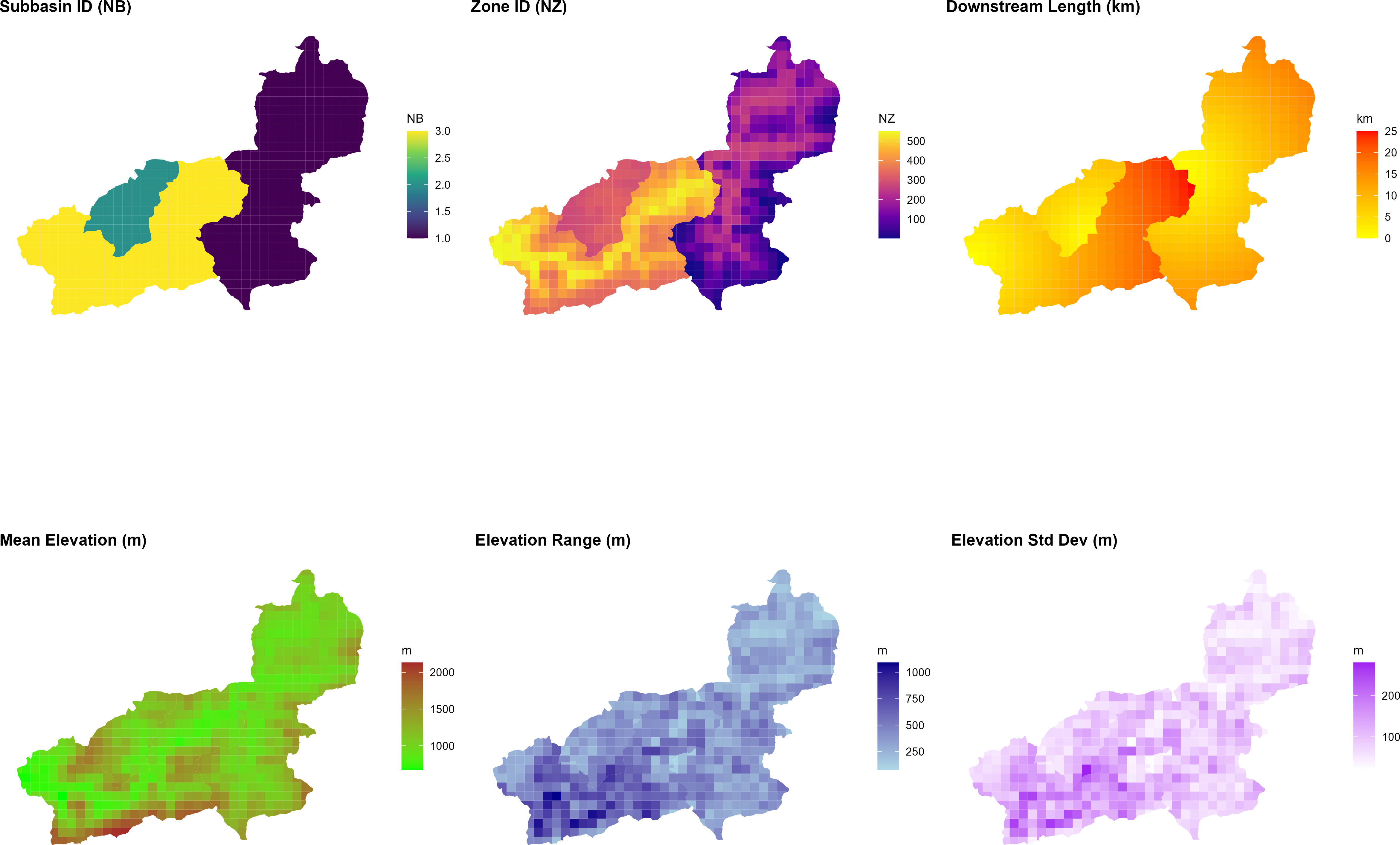
generate_cosero_zones.R. From left to right: subbasin ID (NB), global zone ID (NZ), downstream routing length (km), mean elevation (m), elevation range (m), and elevation standard deviation (m). The three subbasins and their respective elevation gradients are clearly visible. Zone IDs increase continuously across subbasins; the outlet zone of each subbasin has the highest IZ within that subbasin and routes flow to the outlet zone of the downstream subbasin.Step 4: Generating Initial Model Parameters
NoteParameter Raster Downloads
The Austria-wide raster datasets used to derive a priori model parameters are provided below, based on (Zeitfogel et al., 2024; Zeitfogel et al.; 2025). Save all files to the same directory and update the raster_dir path in generate_cosero_parameters.R accordingly.
| File | Parameter(s) derived |
|---|---|
| bodenkarten_cosero_q99q1_lm.tif | Soil storage, field capacity (BOKU soil map) |
| cosero_raster1000.tif | Land use / hydrological response classes |
| ct_at.tif | Snow melt factors |
| etlspcor_at_0_8_1_2.tif | ET slope/aspect correction (ETSLPCOR) |
| Etvegcor.tif | Vegetation ET correction (ETVEGCOR) |
| Intmax.tif | Maximum interception storage (INTMAX) |
| Tmmon.tif | Mean monthly temperature (12 bands, TMMON) |
| waterbodies_corine.tif | Open water mask (CORINE land cover) |
With the zone shapefile in place, initial (a priori) model parameters are extracted from Austria-wide raster maps and assigned to each zone using:
Show/hide: generate_cosero_parameters.R
################################################################################
# Generate COSERO Parameter File from Zone Shapefile and Raster Maps
#
# Input:
#   - Zone shapefile (from generate_cosero_zones.R) with elev_mean and elev_sd
#   - Pre-processed parameter rasters (Austria-wide)
#
# Output:
#   - COSERO parameter file (para_ini.txt)
#   - Shapefile with all parameter attributes
#   - Parameter visualization (4x6 panel plot)
#
# Features:
#   - Dynamic NVAR parameterization based on topographic roughness (elev_sd)
#   - Psychrometric phase split for SNOWTRT/RAINTRT (elevation-dependent)
#   - Elevation-dependent parameters (TCor, PCor, ETSYSCOR, FKFAK, TVAR)
#
# Requirements: R packages sf, terra, dplyr, exactextractr, ggplot2, patchwork
#
# Author: Claude Code / Mathew Herrnegger
# Date: 2026-01
################################################################################

library(sf)
library(terra)
library(dplyr)
library(exactextractr)
library(ggplot2)
library(patchwork)


#===============================================================================
# USER SETTINGS — adapt these paths to your system
#===============================================================================

# Zone shapefile (output from generate_cosero_zones.R)
zones_shp <- "C:/COSERO/MyCatchment/GIS/cosero_zones.shp"

# Directory containing the Austria-wide parameter raster maps
# (provided as course material — contact course instructors)
raster_dir <- "C:/COSERO/MyCatchment/data/parameter_rasters/"

# Output: COSERO parameter input file
output_file <- "C:/COSERO/MyCatchment/input/para_ini.txt"

# Output: Zone shapefile with all parameter attributes (for QC in QGIS)
output_shapefile <- "C:/COSERO/MyCatchment/GIS/cosero_zones_parameters.shp"

#===============================================================================
# DERIVED RASTER PATHS — no changes needed below this line
#===============================================================================

soil_tif      <- file.path(raster_dir, "bodenkarten_cosero_q99q1_lm.tif")
landuse_tif   <- file.path(raster_dir, "cosero_raster1000.tif")
ct_tif        <- file.path(raster_dir, "ct_at.tif")
etslpcor_tif  <- file.path(raster_dir, "etlspcor_at_0_8_1_2.tif")
etvegcor_tif  <- file.path(raster_dir, "Etvegcor.tif")
intmax_tif    <- file.path(raster_dir, "Intmax.tif")
tmmon_tif     <- file.path(raster_dir, "Tmmon.tif")
waterbody_tif <- file.path(raster_dir, "waterbodies_corine.tif")

#===============================================================================
# STEP 1: LOAD ZONE SHAPEFILE
#===============================================================================

cat("Step 1: Loading zone shapefile and aligning CRS...\n")

# Load zones
zones <- st_read(zones_shp, quiet = TRUE)

# Use the first raster to define the "Master CRS"
ref_raster <- rast(soil_tif)
master_crs <- crs(ref_raster)

# Dynamically transform zones to match the raster data
if (st_crs(zones) != st_crs(master_crs)) {
  cat(sprintf("   Aligning zones to raster CRS: %s\n", st_crs(master_crs)$input))
  zones <- st_transform(zones, master_crs)
}

cat(sprintf("   Loaded %d zones\n", nrow(zones)))
cat(sprintf("  Available fields: %s\n", paste(names(zones), collapse = ", ")))


#===============================================================================
# STEP 2: EXTRACT PARAMETERS FROM RASTERS
#===============================================================================

cat("\nStep 2: Extracting parameters from rasters...\n")

# Elevation (use from shapefile)
cat("  Elevation (from shapefile)...\n")
if ("elev_mean" %in% names(zones)) {
  zones$ELEV_ <- round(as.numeric(zones$elev_mean), 1)
} else if ("elev_mn" %in% names(zones)) {
  # Field name might be truncated
  zones$ELEV_ <- round(as.numeric(zones$elev_mn), 1)
} else {
  stop("ERROR: No elevation field found in shapefile. Available fields: ", paste(names(zones), collapse = ", "))
}

# Soil parameters (10 bands: M, KBF, BETA, H1, H2, TAB1, TAB2, TVS1, TVS2, TAB3)
cat("  Soil parameters...\n")
soil <- rast(soil_tif)
soil_names <- c("M_", "KBF_", "BETA_", "H1_", "H2_", "TAB1_", "TAB2_", "TVS1_", "TVS2_", "TAB3_")
for (i in 1:nlyr(soil)) {
  zones[[soil_names[i]]] <- round(exact_extract(soil[[i]], zones, "mean"), 2)
}

# Land use (mode = most common class)
cat("  Land use...\n")
landuse <- rast(landuse_tif)
zones$NC_ <- exact_extract(landuse, zones, "mode")

# Add land use class descriptions
landuse_lookup <- data.frame(
  COSERO_Class = c(1, 2, 3, 4, 5, 6, 7, 8, 9, 10, 999),
  COSERO_text_english = c(
    "Built-up / Urban areas",
    "Arable land / Cropland",
    "Grassland / Pastures",
    "Deciduous / Broad-leaved forest",
    "Coniferous forest",
    "Mixed forest",
    "Sparsely vegetated areas",
    "Glaciers and perpetual snow",
    "Water bodies / Water courses",
    "Wetlands",
    "NO DATA"
  ),
  COSERO_text_german = c(
    "Bebaute Siedlungsflächen",
    "Ackerland",
    "Grünland",
    "Laubwälder",
    "Nadelwälder",
    "Mischwälder",
    "Vegetationsarme Flächen",
    "Gletscher",
    "Wasserflächen",
    "Feuchtgebiete",
    "NO DATA"
  ),
  stringsAsFactors = FALSE
)

# Merge land use descriptions with zones
zones <- merge(zones, landuse_lookup,
               by.x = "NC_", by.y = "COSERO_Class",
               all.x = TRUE, sort = FALSE)

# Display land use summary
cat("  Land use classes found:\n")
landuse_summary <- zones %>%
  st_drop_geometry() %>%
  group_by(NC_, COSERO_text_english) %>%
  summarise(n_zones = n(), .groups = "drop") %>%
  arrange(NC_)
print(landuse_summary)

# Snowmelt factors (2 bands: CTMAX, CTMIN)
cat("  Snowmelt factors...\n")
ct <- rast(ct_tif)
zones$CTMAX_ <- round(exact_extract(ct[[1]], zones, "mean"), 2)
zones$CTMIN_ <- round(exact_extract(ct[[2]], zones, "mean"), 2)

# ETSLPCOR
cat("  ETSLPCOR...\n")
etslpcor <- rast(etslpcor_tif)
zones$ETSLPCOR_ <- round(exact_extract(etslpcor, zones, "mean"), 3)

# ETVEGCOR (12 monthly bands)
cat("  ETVEGCOR (12 months)...\n")
etvegcor <- rast(etvegcor_tif)
for (i in 1:12) {
  zones[[paste0("ETVEGCOR", i, "_")]] <- round(exact_extract(etvegcor[[i]], zones, "mean"), 2)
}

# INTMAX (12 monthly bands)
cat("  INTMAX (12 months)...\n")
intmax <- rast(intmax_tif)
for (i in 1:12) {
  zones[[paste0("INTMAX", i, "_")]] <- round(exact_extract(intmax[[i]], zones, "mean"), 2)
}

# TMMon (12 monthly bands)
cat("  Monthly mean temperature (12 months)...\n")
tmmon <- rast(tmmon_tif)
for (i in 1:12) {
  zones[[paste0("TMMon", i, "_")]] <- round(exact_extract(tmmon[[i]], zones, "mean"), 2)
}

# Waterbody
cat("  Waterbody...\n")
waterbody <- rast(waterbody_tif)
zones$WATERBODY_ <- round(exact_extract(waterbody, zones, "mean"), 2)

#===============================================================================
# STEP 3: ADD ELEVATION-DEPENDENT PARAMETERS
#===============================================================================

cat("\nStep 3: Adding elevation-dependent parameters...\n")

#-------------------------------------------------------------------------------
# Calculate elevation-dependent parameters
#-------------------------------------------------------------------------------

# TCor: Monthly temperature correction (elevation-dependent)
# Based on Hanna's code: higher correction at higher elevations
for (i in 1:12) {
  col_name <- paste0("TCor", i, "_")

  # Base values by month (winter months need less correction)
  base_tcor <- c(0.0, 0.0, 0.0, 0.0, 0.5, 1, 1.25, 1, 0.0, 0.0, 0.0, 0.0)[i]

  zones[[col_name]] <- ifelse(zones$ELEV_ >= 2000, base_tcor, 0)
  zones[[col_name]] <- ifelse(zones$ELEV_ >= 2500, base_tcor + 0, zones[[col_name]])
}

# PCor: Monthly precipitation correction (elevation-dependent)
for (i in 1:12) {
  col_name <- paste0("PCor", i, "_")

  # Higher correction in winter months at high elevations
  if (i %in% c(1, 2, 3, 11, 12)) {
    zones[[col_name]] <- ifelse(zones$ELEV_ >= 2500, 2.0,
                         ifelse(zones$ELEV_ >= 2000, 1.5,
                         ifelse(zones$ELEV_ >= 1500, 1.4, 1.2)))
  } else if (i %in% c(4, 5, 9, 10)) {
    zones[[col_name]] <- ifelse(zones$ELEV_ >= 2500, 1.8,
                         ifelse(zones$ELEV_ >= 2000, 1.5,
                         ifelse(zones$ELEV_ >= 1500, 1.2, 1.1)))
  } else {
    zones[[col_name]] <- ifelse(zones$ELEV_ >= 2500, 1.8,
                         ifelse(zones$ELEV_ >= 2000, 1.5,
                         ifelse(zones$ELEV_ >= 1500, 1.2, 1.1)))
  }
}

# ETSYSCOR: Systematic ET correction (elevation-dependent, same for all months)
etsyscor_value <- round(0.000165 * zones$ELEV_ + 1.039757, 3)
for (i in 1:12) {
  zones[[paste0("ETSYSCOR", i, "_")]] <- etsyscor_value
}


# TVAR: Temperature variability (elevation-dependent)
tvar_elev_high <- 1000    # Elevation above which TVAR = tvar_high
tvar_elev_low <- 500      # Elevation below which TVAR = tvar_low
tvar_high <- 0          # TVAR value at high elevation
tvar_low <- 0          # TVAR value at low elevation

zones$TVAR_ <- ifelse(zones$ELEV_ > tvar_elev_high, tvar_high,
               ifelse(zones$ELEV_ < tvar_elev_low, tvar_low,
                      round((zones$ELEV_ - tvar_elev_low) / (tvar_elev_high - tvar_elev_low) *
                            (tvar_high - tvar_low) + tvar_low, 2)))

#-------------------------------------------------------------------------------
# NVAR: Sub-grid snow variability based on composite topographic roughness
# Physical Background: Snow depth varies on sub-grid scale due to wind drifting,
# avalanching, and solar shading. Represented by log-normal distribution.
# NVAR is the coefficient of variation.
#
# Logic: We combine Elev_SD (vertical capacity for drifts) with Slope (mechanical
# force for redistribution). We apply equal weights to Elev_SD and mean slope.
#-------------------------------------------------------------------------------

# Configuration parameters
nvar_min <- 0.05           # Minimum NVAR (flattest cell, uniform snow cover)
nvar_max <- 2.0           # Maximum NVAR (most rugged cell, heavy drifting/scouring)
weight_sd <- 0.3          # Weight for elevation SD (vertical capacity)
weight_slope <- 0.7       # Weight for slope (mechanical redistribution force)

# Get elevation SD from shapefile (handle field name truncation)
if ("elev_sd" %in% names(zones)) {
  e_sd <- as.numeric(zones$elev_sd)
} else {
  cat("  WARNING: No elev_sd field found - using default for NVAR\n")
  e_sd <- rep(50, nrow(zones))  # Default SD
}

# Get slope from shapefile (handle field name truncation)
if ("slop_mn" %in% names(zones)) {
  s_mn <- as.numeric(zones$slop_mn)
} else {
  cat("  WARNING: No slope field found - using elev_sd only for NVAR\n")
  s_mn <- rep(0, nrow(zones))  # Default slope
}

# Log-transform SD: Accounts for 'topographic saturation' (peaks vs hills)
log_rough <- log(e_sd + 1)

# Normalize both indicators to a 0-1 scale
norm_sd    <- (log_rough - min(log_rough)) / (max(log_rough) - min(log_rough))
norm_slope <- (s_mn - min(s_mn)) / (max(s_mn) - min(s_mn))

# Weighted Composite: SD is the primary driver, Slope is the modifier
composite_rough <- (norm_sd * weight_sd) + (norm_slope * weight_slope)

# Scale to COSERO range [nvar_min, nvar_max]
zones$NVAR_ <- round((composite_rough * (nvar_max - nvar_min)) + nvar_min, 2)

cat(sprintf("  NVAR range: %.2f - %.2f (composite: %.0f%% elev_sd + %.0f%% slope)\n",
            min(zones$NVAR_), max(zones$NVAR_), weight_sd * 100, weight_slope * 100))

#-------------------------------------------------------------------------------
# RAINTRT / SNOWTRT: Psychrometric phase split thresholds
# Physical Background: Phase of precipitation depends on snowflake energy balance.
# In high-alpine air (lower pressure/humidity), snowflakes stay frozen at higher
# temperatures due to latent heat loss from sublimation (Wet-Bulb Effect).
#-------------------------------------------------------------------------------

# Identify study-area extremes for adaptive scaling
max_elev <- max(zones$ELEV_)
min_elev <- min(zones$ELEV_)

# Normalize elevation to 0-1 scale
zones$rel_elev <- (zones$ELEV_ - min_elev) / (max_elev - min_elev)

#-------------------------------------------------------------------------------
# Wet-Bulb Depression Approach:
# Physical basis: At higher elevations, lower atmospheric pressure and humidity
# cause greater evaporative cooling of falling precipitation (wet-bulb effect).
# This shifts BOTH thresholds upward by the same amount, maintaining a constant
# transition window across all elevations.
#-------------------------------------------------------------------------------

# Configuration parameters
base_snow_temp <- -1.0         # Snow threshold at valley floor (°C)
base_rain_temp <- 2.0          # Rain threshold at valley floor (°C)
wb_depression_max <- 1.5       # Maximum wet-bulb depression at highest elevation (°C)

# Wet-bulb depression increases linearly with elevation
# (lower humidity/pressure at altitude)
wb_depression <- zones$rel_elev * wb_depression_max

# Both thresholds shift upward with elevation
zones$SNOWTRT_ <- round(base_snow_temp + wb_depression, 1)
zones$RAINTRT_ <- round(base_rain_temp + wb_depression, 1)

# Transition window remains constant: base_rain_temp - base_snow_temp
window_width <- base_rain_temp - base_snow_temp

cat(sprintf("  Wet-bulb depression: %.1f °C at peak elevation\n", wb_depression_max))
cat(sprintf("  Constant transition window: %.1f °C\n", window_width))

#-------------------------------------------------------------------------------
# Summary output
#-------------------------------------------------------------------------------
cat(sprintf("  SNOWTRT range: %.1f - %.1f °C\n", min(zones$SNOWTRT_), max(zones$SNOWTRT_)))
cat(sprintf("  RAINTRT range: %.1f - %.1f °C\n", min(zones$RAINTRT_), max(zones$RAINTRT_)))


#-------------------------------------------------------------------------------
# RAINCOR / SNOWCOR: Phase fraction correction factors
# Default set to 1.0 (no correction). Can be adjusted for systematic biases.
#-------------------------------------------------------------------------------

zones$RAINCOR_ <- 1.0
zones$SNOWCOR_ <- 1.0

# Remove temporary column
zones$rel_elev <- NULL


# FKFAK: Field capacity factor aboove which ETA=ETP (elevation-dependent)
fkfak_high <- 0.4         # FKFAK value at highest elevation
fkfak_low <- 0.7          # FKFAK value at lowest elevation
zones$FKFAK_ <- round((zones$ELEV_ - min(zones$ELEV_)) /
                      (max(zones$ELEV_) - min(zones$ELEV_)) * (fkfak_high - fkfak_low) + fkfak_low, 2)

#===============================================================================
# STEP 4: ADD DEFAULT PARAMETERS
#===============================================================================

cat("\nStep 4: Adding default parameters...\n")

# Zone structure (use from shapefile)
zones$NB_ <- as.integer(zones$NB)
zones$NZ_ <- as.integer(zones$NZ)
zones$IZ_ <- as.integer(zones$IZ)
zones$TONZ_ <- as.integer(zones$ToNZ)

# Coordinates (convert to -999 if missing, as in template)
# Use existing X_COORD and Y_COORD fields from shapefile
zones$X_COORD <- ifelse(is.na(zones$X_COORD), -999, as.numeric(zones$X_COORD))
zones$Y_COORD <- ifelse(is.na(zones$Y_COORD), -999, as.numeric(zones$Y_COORD))

# Default values for other parameters
# DFZON: Zone area in km² (from shapefile)
if ("area_km2" %in% names(zones)) {
  zones$DFZON_ <- as.numeric(zones$area_km2)
} else if ("are_km2" %in% names(zones)) {
  zones$DFZON_ <- as.numeric(zones$are_km2)
} else {
  cat("  No area field found - calculating from geometry...\n")
  # Calculate area from geometry (CRS is in meters, convert to km²)
  zones$DFZON_ <- as.numeric(st_area(zones)) / 1e6
}

zones$THRT_ <- 0
zones$FK_ <- 1
zones$PWP_ <- 0

# Additional parameters
zones$TAB4_ <- 1.3763
zones$TAB5_ <- 2.357

# Monthly DAYSDRY (12 months) - default 0
for (i in 1:12) {
  zones[[paste0("DAYSDRY", i, "_")]] <- 0
}

# Monthly DAYSWET (12 months) - default 1
for (i in 1:12) {
  zones[[paste0("DAYSWET", i, "_")]] <- 1
}

# Initial state variables
zones$KMELTRINI_ <- 0
zones$KSHINI_ <- 0
zones$KSWINI_ <- 0
zones$TSOILINI_ <- 5
zones$BW0INI_ <- 0.7
zones$BW1INI_ <- 0
zones$BW2INI_ <- 25
zones$BW3INI_ <- 250
zones$BW4INI_ <- 0

# Additional parameters
zones$BAREGR_ <- 0
zones$CTNeg_ <- 1
zones$CTRed_ <- 0.7
zones$DWHCAP_ <- 0
zones$EVPNS_ <- 0.7
zones$EVPSNO_ <- 0.3
zones$NSRHOMAX_ <- 0.3
zones$PEX2_ <- 9999
zones$PEX3_ <- 9999
zones$SETCON_ <- 0.2
zones$SNOWDET_ <- 1
zones$SOILTYPE_ <- 1
zones$SRHOMAX_ <- 0.45
zones$TSOILMAX_ <- 15
zones$TSOILMIN_ <- -5
zones$UADJ_ <- 2
zones$WHCAP_ <- 0.05
zones$SPARE1_ <- 1
zones$SPARE2_ <- 1
zones$SPARE3_ <- 1

# Glacier parameters (defaults, no glaciers in Wildalpen)
zones$GLAC_CT_ <- 1
zones$GLAC_GLFAKT_ <- 0.02
zones$GLAC_ICECOV_ <- 0
zones$GLAC_TAB_ <- 8
zones$GLAC_INI_ <- 99999

# Diversion parameters (no diversions)
zones$Div_TONZ <- zones$TONZ_
zones$QDIV_LT_ <- 999
zones$QDIV_UT_ <- 999
zones$QDIV_RATIO_ <- 0

#===============================================================================
# STEP 5: BUILD PARAMETER DATA FRAME
#===============================================================================

cat("\nStep 5: Building parameter data frame...\n")

# Define column order (COSERO format - matches template exactly)
param_cols <- c(
  # Zone structure
  "NB_", "IZ_", "NZ_", "TONZ_", "Div_TONZ", "QDIV_LT_", "QDIV_UT_", "QDIV_RATIO_",
  # Coordinates and basic info
  "X_COORD", "Y_COORD", "WATERBODY_", "DFZON_", "ELEV_", "NC_",
  # ET and snowmelt parameters
  "ETSLPCOR_", "CTMAX_", "CTMIN_", "NVAR_",
  # Precipitation and snow parameters
  "RAINTRT_", "RAINCOR_", "SNOWCOR_", "SNOWTRT_", "THRT_",
  # Soil parameters
  "M_", "FK_", "PWP_", "KBF_", "BETA_", "FKFAK_",
  "H1_", "H2_", "TAB1_", "TAB2_", "TVS1_", "TVS2_", "TAB4_", "TAB3_", "TAB5_",
  # Monthly precipitation correction
  paste0("PCor", 1:12, "_"),
  # Monthly temperature correction
  paste0("TCor", 1:12, "_"),
  # Monthly mean temperature
  paste0("TMMon", 1:12, "_"),
  # Monthly interception maximum
  paste0("INTMAX", 1:12, "_"),
  # Monthly ET vegetation correction
  paste0("ETVEGCOR", 1:12, "_"),
  # Monthly dry days
  paste0("DAYSDRY", 1:12, "_"),
  # Monthly wet days
  paste0("DAYSWET", 1:12, "_"),
  # Monthly ET systematic correction
  paste0("ETSYSCOR", 1:12, "_"),
  # Initial state variables
  "KMELTRINI_", "KSHINI_", "KSWINI_", "TSOILINI_",
  "BW0INI_", "BW1INI_", "BW2INI_", "BW3INI_", "BW4INI_",
  # Additional parameters
  "BAREGR_", "CTNeg_", "CTRed_", "DWHCAP_", "EVPNS_", "EVPSNO_",
  "NSRHOMAX_", "PEX2_", "PEX3_", "SETCON_", "SNOWDET_", "SOILTYPE_",
  "SRHOMAX_", "TSOILMAX_", "TSOILMIN_", "TVAR_", "UADJ_", "WHCAP_",
  "SPARE1_", "SPARE2_", "SPARE3_",
  # Glacier parameters
  "GLAC_CT_", "GLAC_GLFAKT_", "GLAC_ICECOV_", "GLAC_TAB_", "GLAC_INI_"
)

# Create output data frame
para_df <- st_drop_geometry(zones)
para_df <- para_df[order(para_df$NZ_), ]

# Check which columns are missing
missing_cols <- setdiff(param_cols, names(para_df))
if (length(missing_cols) > 0) {
  cat(sprintf("  WARNING: %d columns missing:\n", length(missing_cols)))
  cat(sprintf("    %s\n", paste(missing_cols, collapse = ", ")))
  cat("  Setting missing columns to 0...\n")
  for (col in missing_cols) {
    para_df[[col]] <- 0
  }
}

# Select and order columns
para_out <- para_df[, param_cols]

# Replace NA with defaults
para_out[is.na(para_out)] <- 0

cat(sprintf("  %d zones, %d parameters\n", nrow(para_out), ncol(para_out)))

#===============================================================================
# STEP 6: WRITE PARAMETER FILE
#===============================================================================

cat("\nStep 6: Writing parameter file...\n")

# Create output directory
output_dir <- dirname(output_file)
if (!dir.exists(output_dir)) {
  dir.create(output_dir, recursive = TRUE)
}

# Prepare header line (matches template format)
n_zones <- nrow(para_out)
n_subbasins <- length(unique(para_out$NB_))
current_time <- format(Sys.time(), "%H:%M")
current_year <- format(Sys.Date(), "%Y")

header_line1 <- paste("COSERO-Wildalpen", current_time, n_zones, n_subbasins, current_year, sep = "\t")
header_line2 <- paste(names(para_out), collapse = "\t")

# Write file
con <- file(output_file, "w")
writeLines(header_line1, con)
writeLines(header_line2, con)
write.table(para_out, con, sep = "\t", row.names = FALSE, col.names = FALSE, quote = FALSE)
close(con)

cat(sprintf("  Written: %s\n", output_file))

#===============================================================================
# STEP 7: EXPORT SHAPEFILE WITH ALL ATTRIBUTES
#===============================================================================

cat("\nStep 7: Exporting shapefile with all attributes...\n")

# Reorder zones by NZ for consistency
zones_export <- zones[order(zones$NZ), ]

# Rename long field names for shapefile compatibility (10 char limit)
# COSERO_text_english -> LU_name_en (Land Use name english)
# COSERO_text_german  -> LU_name_de (Land Use name german)
if ("COSERO_text_english" %in% names(zones_export)) {
  names(zones_export)[names(zones_export) == "COSERO_text_english"] <- "LU_name_en"
}
if ("COSERO_text_german" %in% names(zones_export)) {
  names(zones_export)[names(zones_export) == "COSERO_text_german"] <- "LU_name_de"
}

# Create output directory if it doesn't exist
output_shp_dir <- dirname(output_shapefile)
if (!dir.exists(output_shp_dir)) {
  dir.create(output_shp_dir, recursive = TRUE)
  cat(sprintf("  Created directory: %s\n", output_shp_dir))
}

# Write shapefile (includes all attributes: parameters + land use descriptions)
st_write(zones_export, output_shapefile, delete_dsn = TRUE, quiet = FALSE)

cat(sprintf("  Written: %s\n", output_shapefile))
cat(sprintf("  Attributes: %d (including LU_name_en, LU_name_de)\n",
            ncol(st_drop_geometry(zones_export))))


#===============================================================================
# STEP 8: CALCULATE MONTHLY AVERAGES AND PLOT PARAMETERS
#===============================================================================

cat("\nStep 8: Creating parameter plots...\n")

# Calculate monthly averages (drop geometry for numeric operations)
zones_df <- st_drop_geometry(zones)
zones$PCor_mean <- rowMeans(zones_df[, paste0("PCor", 1:12, "_")], na.rm = TRUE)
zones$TCor_mean <- rowMeans(zones_df[, paste0("TCor", 1:12, "_")], na.rm = TRUE)
zones$TMMon_mean <- rowMeans(zones_df[, paste0("TMMon", 1:12, "_")], na.rm = TRUE)
zones$INTMAX_mean <- rowMeans(zones_df[, paste0("INTMAX", 1:12, "_")], na.rm = TRUE)
zones$ETVEGCOR_mean <- rowMeans(zones_df[, paste0("ETVEGCOR", 1:12, "_")], na.rm = TRUE)
zones$ETSYSCOR_mean <- rowMeans(zones_df[, paste0("ETSYSCOR", 1:12, "_")], na.rm = TRUE)

# Function to create parameter plot
create_param_plot <- function(data, var_name, plot_title, color_low = "yellow", color_high = "red") {
  ggplot(data) +
    geom_sf(aes(fill = .data[[var_name]]), color = NA) +
    scale_fill_gradient(low = color_low, high = color_high, name = "") +
    labs(title = plot_title) +
    theme_minimal() +
    theme(
      axis.text = element_blank(),
      axis.ticks = element_blank(),
      panel.grid = element_blank(),
      plot.title = element_text(size = 10, face = "bold"),
      legend.title = element_text(size = 8),
      legend.text = element_text(size = 7),
      legend.key.height = unit(0.4, "cm"),
      legend.key.width = unit(0.3, "cm")
    )
}

# Define plot specifications (variable, title, color_low, color_high)
# Organized in logical groups
plot_specs <- list(
  # Row 1: Temperature and snow parameters
  list("CTMAX_", "CTMAX (Snowmelt factor max)", "lightyellow", "red"),
  list("CTMIN_", "CTMIN (Snowmelt factor min)", "lightyellow", "darkorange"),
  list("RAINTRT_", "RAINTRT (Rain threshold °C)", "lightblue", "blue"),
  list("SNOWTRT_", "SNOWTRT (Snow threshold °C)", "lightcyan", "darkblue"),

  # Row 2: Snow / Soil parameters (part 1)
  list("NVAR_", "NVAR (Snow variability)", "white", "gray30"),
  list("M_", "M (Soil depth (effective))", "wheat", "brown"),
  list("KBF_", "KBF (Soil percolation coef.)", "lightgreen", "darkgreen"),
  list("BETA_", "BETA (Soil exponent)", "lightyellow", "darkorange"),

  # Row 3: Soil parameters (part 2)
  list("H1_", "H1 (Threshold fast runoff tank)", "tan1", "tan4"),
  list("H2_", "H2 (Threshold interflow tank)", "tan1", "tan4"),
  list("TAB1_", "TAB1 (Fast runoff coef.)", "lightsteelblue1", "steelblue4"),
  list("TAB2_", "TAB2 (Interflow coef.)", "lightsteelblue1", "steelblue4"),

  # Row 4: Soil parameters (part 3) + NVAR
  list("TVS1_", "TVS1 (Fast runoff perc.)", "lavender", "purple4"),
  list("TVS2_", "TVS2 (Interflow perc.)", "lavender", "purple4"),
  list("TAB3_", "TAB3 (Baseflow coef. 3)", "lightsteelblue1", "steelblue4"),
  list("PCor_mean", "PCor mean (Precip. cor.)", "honeydew", "forestgreen"),

  # Row 5: Monthly averages (part 1)
  list("TCor_mean", "TCor mean (Temp. cor.)", "mistyrose", "red3"),
  list("TMMon_mean", "TMMon mean (Mean temp.)", "lightyellow", "orangered"),
  list("INTMAX_mean", "INTMAX mean (Intercept.)", "lightcyan", "cyan4"),
  list("ETVEGCOR_mean", "ETVEGCOR mean (ET veg. cor)", "palegreen", "green4"),

  # Row 6: Monthly averages (part 2)
  list("ETSYSCOR_mean", "ETSYSCOR mean (ET sys. cor)", "lemonchiffon", "yellow4"),
  list("FKFAK_", "FKFAK (Field capacity factor for ET)", "lightgoldenrod", "goldenrod4")
)

# Create all plots
plots <- lapply(plot_specs, function(spec) {
  create_param_plot(zones, spec[[1]], spec[[2]], spec[[3]], spec[[4]])
})

# Combine into 4 columns x 6 rows layout
combined_plot <- wrap_plots(plots, ncol = 4, nrow = 6)

# Save plot
plot_file <- gsub("\\.shp$", "_parameters.png", output_shapefile)
ggsave(plot_file, combined_plot, width = 16, height = 17, dpi = 300, bg = "white")
cat(sprintf("  Plot saved: %s\n", plot_file))

# Display plot
print(combined_plot)

#===============================================================================
# SUMMARY
#===============================================================================

cat("\n=== SUMMARY ===\n")
cat(sprintf("Zones: %d\n", nrow(para_out)))
cat(sprintf("Subbasins: %d\n", length(unique(para_out$NB_))))
cat(sprintf("Parameters: %d\n", ncol(para_out)))
cat(sprintf("Elevation range: %.0f - %.0f m\n", min(para_out$ELEV_), max(para_out$ELEV_)))

cat("\nDynamic parameterization (elevation + topography):\n")
cat(sprintf("  NVAR (snow variability): %.2f - %.2f (based on elev_sd)\n",
            min(para_out$NVAR_), max(para_out$NVAR_)))
cat(sprintf("  SNOWTRT (snow threshold): %.1f - %.1f °C (psychrometric effect)\n",
            min(para_out$SNOWTRT_), max(para_out$SNOWTRT_)))
cat(sprintf("  RAINTRT (rain threshold): %.1f - %.1f °C (psychrometric effect)\n",
            min(para_out$RAINTRT_), max(para_out$RAINTRT_)))

cat("\nOutput files:\n")
cat(sprintf("  Parameter file (para_ini.txt): %s\n", output_file))
cat(sprintf("  Shapefile with attributes: %s\n", output_shapefile))
cat(sprintf("  Parameter plots: %s\n", plot_file))

cat("\nDone!\n")
Parameters are extracted from pre-processed raster datasets covering soil properties, land use, snowmelt factors, evapotranspiration corrections, and interception. Several parameters are derived dynamically based on elevation and topographic roughness (elevation standard deviation within a zone):
- NVAR (snow spatial variability) — scaled from topographic roughness (elevation SD + slope), reflecting sub-grid snow redistribution by wind and avalanches.
- SNOWTRT / RAINTRT (precipitation phase thresholds) — shifted upward at higher elevations to account for the wet-bulb depression effect (lower pressure and humidity cause snowflakes to remain frozen at warmer temperatures).
- PCor / TCor (precipitation and temperature corrections) — elevation-dependent monthly correction factors.
- ETSYSCOR (systematic ET correction) — linearly scaled with elevation.
- FKFAK (field capacity factor for ET) — decreases with elevation, reflecting drier, more permeable high-alpine soils.
The script produces three outputs:
para_ini.txt— The COSERO parameter input file, tab-delimited, one row per zone.- Zone shapefile with all parameter attributes — for visual inspection and quality control in QGIS.
- Parameter maps — a 4 × 6 panel plot showing the spatial distribution of all key parameters across the catchment.
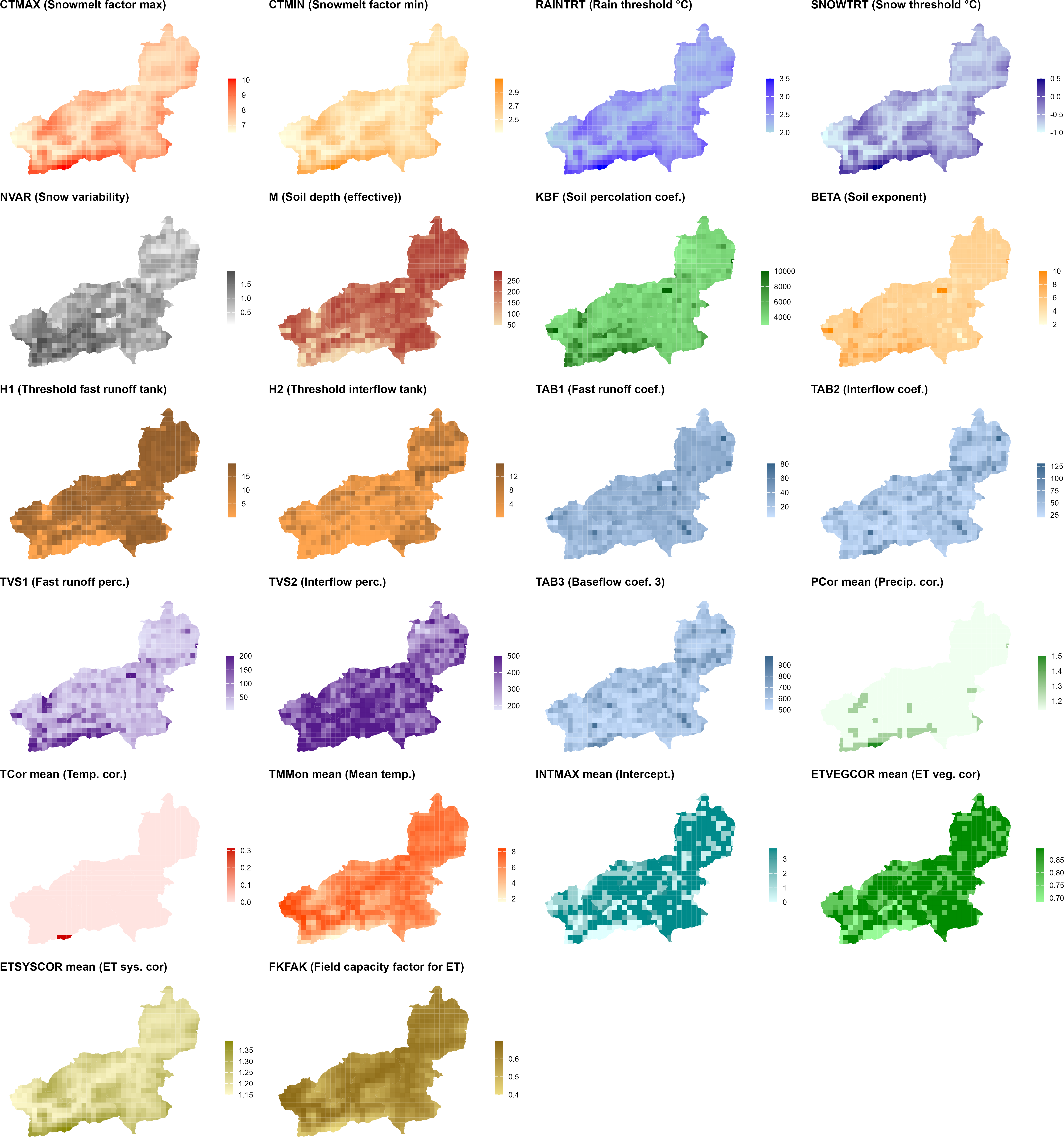
generate_cosero_parameters.R. Each panel shows one parameter. The top rows cover snowmelt factors (CTMAX, CTMIN), precipitation phase thresholds (RAINTRT, SNOWTRT), and snow variability (NVAR). The middle rows show soil and runoff generation parameters derived from the BOKU soil map (M, KBF, BETA, H1, H2, TAB1, TAB2, TVS1, TVS2, TAB3). The bottom rows display elevation-dependent correction factors (PCor, TCor, ETSYSCOR) and vegetation and interception corrections (ETVEGCOR, INTMAX, FKFAK). All parameters are spatially differentiated across zones — patterns closely follow elevation and subbasin structure.
TipUser-configurable settings in
generate_cosero_parameters.R
The script is designed to be adapted to your catchment. The most important settings to review and adjust are:
Paths (top of script)
zones_shp— path to your zone shapefile (output of Step 3)raster_dir— directory containing the Austria-wide parameter rastersoutput_file— where the COSERO parameter file (para_ini.txt) will be writtenoutput_shapefile— where to save the zone shapefile with all parameter attributes
Elevation-dependent snow parameters
base_snow_temp,base_rain_temp— precipitation phase thresholds (°C) at valley floor; sensible defaults are −1 and 2 °C respectivelywb_depression_max— maximum wet-bulb depression at the highest elevation (°C); controls how much the thresholds shift upward in alpine zones
Snow spatial variability (NVAR)
nvar_min,nvar_max— range of the NVAR coefficient of variation; defaults are 0.05–2.0weight_sd,weight_slope— relative contribution of elevation SD vs. mean slope to the composite topographic roughness index; must sum to 1
Precipitation correction factors (PCor — 12 monthly values)
PCor is a monthly multiplicative factor applied to zone precipitation before phase partitioning. It is set as a step-function of elevation, with separate values for three seasonal groups and current settings for Wildalpen:
| Season | Months | < 1500 m | 1500–2000 m | 2000–2500 m | ≥ 2500 m |
|---|---|---|---|---|---|
| Winter | Jan, Feb, Mar, Nov, Dec | 1.2 | 1.4 | 1.5 | 2.0 |
| Transitional | Apr, May, Sep, Oct | 1.1 | 1.2 | 1.5 | 1.8 |
| Summer | Jun, Jul, Aug | 1.1 | 1.2 | 1.5 | 1.8 |
Higher values in winter reflect gauge undercatch of solid precipitation, which is strongest at high elevations and during cold months. The elevation thresholds (1500, 2000, 2500 m) and the correction values in each cell are all freely adjustable in the script — modify the ifelse chains in the PCor section of Step 3. For your own catchment, start with PCor = 1.0 for all months and elevation bands (no correction). Introduce corrections only after inspecting initial model runs: systematic water balance errors (simulated runoff consistently too low) or an implausible seasonal pattern (underestimated winter flows, good summer performance) are typical indicators that gauge undercatch is influencing the results.
Temperature correction factors (TCor — 12 monthly values)
TCor is a monthly additive correction (in °C) applied to zone temperature inputs. It accounts for local temperature deviations not captured by the gridded SPARTACUS product, for example in deep valley situations or at exposed ridge stations. In the script and for Wildalpen, corrections are only applied above 2000 m, using a fixed monthly base vector:
| J | F | M | A | M | J | J | A | S | O | N | D |
|---|---|---|---|---|---|---|---|---|---|---|---|
| 0 | 0 | 0 | 0 | +0.5 | +1.0 | +1.25 | +1.0 | 0 | 0 | 0 | 0 |
The summer-only positive corrections compensate for a known deficiency of the degree-day method when applied at a daily time step: mean daily temperature does not capture the full energy available for snowmelt — for example from direct solar radiation on clear-sky high-alpine days or from wind-driven sensible heat flux. Without a correction, the model tends to underestimate melt rates and allows unrealistic snow accumulations (“snow towers”) to build up in high-alpine zones (Haberl, 2021). Zones below 2000 m receive TCor = 0. For your own catchment, start with all values set to zero and only introduce corrections after inspecting simulated vs. observed snow cover during spring and summer.
ET and field capacity
fkfak_high,fkfak_low— FKFAK values at the highest and lowest elevation; lower values at high elevation reflect drier, more permeable alpine soils- ETSYSCOR is computed from a linear regression on elevation (
0.000165 × ELEV + 1.04); adjust the coefficients if your catchment has a different climate–elevation relationship
Default and initial state parameters (Step 4 of the script)
- Initial storage values (
BW0INI_,BW2INI_,BW3INI_, etc.) are set to physically plausible cold-start defaults. If you have a warm start from a previous run (statevar.dmp), these values are overridden at runtime. - Glacier parameters (
GLAC_CT_,GLAC_ICECOV_, etc.) default to zero ice cover — adjust if your catchment contains glaciers. - Routing coefficients
TAB4_andTAB5_are set to Wildalpen-specific defaults; adjust for your catchment after reviewing sensitivity analysis results (Module 3).
ImportantBack up your parameter file
Before modifying para_ini.txt — manually or via script — save a copy:
file.copy(
  from      = "C:/COSERO/MyCatchment/input/para_ini.txt",
  to        = "C:/COSERO/MyCatchment/input/para_ini_backup.txt",
  overwrite = FALSE
)
This is especially important before running automatic calibration in Module 4, where the optimiser writes a new parameter file to the project directory.
TipCOSERO Terminology
- NB: Subbasin index - represents major drainage areas
- NZ: Zone index - represents HRUs within subbasins (elevation bands, land cover classes)
- NBASIN: Total number of subbasins
- IZONE: Total number of zones per subbasin
NoteThe Parameter Estimation Problem
Model parameter estimation remains one of the chief challenges in distributed hydrological modelling. Many parameters represent complex, spatially heterogeneous land surface properties — soil texture, macropore density, vegetation interception or root depth, snow redistribution — that cannot be measured directly at the scale of a model zone or grid cell. This means that even a carefully prepared para_ini.txt will rarely produce a well-calibrated model straight away.
Why is this fundamentally hard?
Spatially distributed models must specify parameter values at every zone or grid cell — if a model has 10 parameters and 10,000 grid cells, there are 100,000 unknowns to determine from a comparatively small number of discharge observations. This is a severely underdetermined and ill-posed problem (Gupta, 2026). A common solution is regularization: linking parameters to observable landscape attributes (soil texture, topography, land cover) through property-to-parameter (P2P) relationships — in hydrology often called pedotransfer functions or transfer functions. This reduces the unknowns dramatically, but shifts the problem: the mathematical form of these relationships is rarely known and is typically specified by expert judgement and trial-and-error. The tension between identifiability (can the data distinguish between different parameter sets?) and over-parameterisation is a central challenge you will explore further in Module 3 through sensitivity analysis, and in Module 4 through automatic calibration.
What a priori values are good for
Despite these limitations, raster-derived a priori parameters serve two important purposes:
- Physically plausible starting point — parameters are in a realistic range and spatially differentiated (e.g. higher elevation zones have lower field capacity, higher snow variability), which prevents the optimizer from getting stuck in physically meaningless regions of parameter space.
- Constraint for calibration — knowing the physically reasonable range of each parameter helps define search bounds for automatic calibration (Module 3) and provides a sanity check on optimised values.
A caveat on interpretation
The resulting parameter fields — whether raster-derived or optimised — should not be interpreted as true point-scale physical properties. In distributed models, parameters are effective, conceptual quantities that may compensate for structural model deficiencies and scale mismatches between data and model domains. Subsurface heterogeneity and the scarcity of direct observations further limit validation. Parameter values are therefore best understood as effective fields implied by the chosen transfer functions, model structure, and available data (Feigl et al., 2026). Improving physical interpretability is possible but typically requires additional constraints such as remotely sensed soil moisture or snow cover data incorporated explicitly into the calibration objective.
Recent advances
Feigl et al. (2026) demonstrate that modern deep learning — specifically a text-generating variational autoencoder trained to generate physically interpretable symbolic equations — can learn plausible P2P relationships directly from input–output data and spatially extensive measurements of physical properties. This approach converts the high-dimensional discrete search over mathematical symbol combinations into a tractable continuous optimization problem, offering a principled alternative to hand-crafted transfer functions.
Part 2: Meteorological Inputs
How COSERO Processes Meteorological Inputs
Before looking into meterological input data preparation, it’s important to understand how COSERO internally processes the meteorological inputs you provide.
Precipitation Partitioning: Rainfall and Snow
For every time step, COSERO separates the precipitation input into liquid rainfall and snowfall based on air temperature. To account for mixed precipitation events (sleet), a linear transition function is used between an upper and lower temperature threshold.
The model parameters SNOWTRT and RAINTRT define the temperature boundaries:
- Below
SNOWTRT: all precipitation falls as snow - Above
RAINTRT: all precipitation is liquid rainfall - Between thresholds: linear interpolation (mixed precipitation)
The equations include multiplicative correction factors for total precipitation (PCOR), liquid precipitation (RAINCOR), and solid precipitation (SNOWCOR):
Step 1: Apply general precipitation correction
\[ PZON_t = P_t \times PCOR_{NM} \tag{1}\]
Step 2: Partition based on temperature
If \(T_t > RAINTRT\) (all rain): \[ PRAIN_t = PZON_t \times RAINCOR \tag{2}\] \[ PSNOW_t = 0 \]
If \(SNOWTRT < T_t < RAINTRT\) (mixed precipitation): \[ PRAIN_t = PZON_t \times \left(\frac{T_t - SNOWTRT}{RAINTRT - SNOWTRT}\right) \times RAINCOR \tag{3}\] \[ PSNOW_t = (PZON_t - PRAIN_t) \times SNOWCOR \tag{4}\]
If \(T_t < SNOWTRT\) (all snow): \[ PRAIN_t = 0 \] \[ PSNOW_t = PZON_t \times SNOWCOR \tag{5}\]
| Parameter | Description | Unit |
|---|---|---|
PCOR |
Monthly correction factor for precipitation | - |
RAINCOR |
Correction factor for liquid precipitation (systematic errors) | - |
SNOWCOR |
Correction factor for snow (e.g., undercatch of snow events) | - |
RAINTRT |
Temperature above which precipitation is pure rain | °C |
SNOWTRT |
Temperature below which precipitation is pure snow | °C |
ImportantPrecipitation Undercatch
Precipitation undercatch is one of the most significant sources of systematic error in alpine hydrology. Solid precipitation measurements from rain gauges systematically underestimate actual snowfall due to wind-induced deflection of snowflakes around the gauge orifice, wetting losses, and evaporation. In complex, high-alpine terrain — where precipitation gradients are steep and gauging networks are sparse — these biases can be substantial, with undercatch corrections exceeding 50 % in exposed locations (Herrnegger et al., 2015, 2018; Maier et al., 2026; Pulka et al., 2024). Beyond gauge undercatch, occult precipitation — dew, fog drip, and rime deposition — is typically not measured at standard meteorological stations, yet can contribute substantially to the local water budget, particularly at high elevations and in forested areas.
The SNOWCOR, RAINCORand PCOR parameter in COSERO (often > 1.0) provide a monthly, zone-level correction for this systematic undercatch. Estimating appropriate values is non-trivial and remains an active research area at BOKU-HyWa, including approaches based on inverse modelling (Herrnegger et al., 2015), spatial interpolation of corrected gridded products (Maier et al., 2026), and satellite-based snow observations assimilated into hydrological models (Pulka et al., 2025).
Potential Evapotranspiration
The potential evapotranspiration (ETP) represents the upper boundary condition for the soil water balance simulation. It is the rate at which evapotranspiration would occur from a surface with unlimited water supply.
COSERO uses the Thornthwaite method for estimation of potential evapotranspiration if no external ETP data is provided. This temperature-based approach estimates ETP as a function of mean monthly temperature and a heat index.
\[ ETP_t = \left[ 17.6 \times \left( \frac{10 \times \max(T_t, 0)}{J} \right)^a \times f_{geo,NM} \right] \times \max\left(0, \min\left(1, 1 - \frac{PZON_t}{EVPNS}\right)\right) \times ETSYSCOR \times ETSLPCOR \tag{6}\]
where the heat index \(J\) and exponent \(a\) are calculated from long-term mean monthly temperatures (TMMON):
\[ J = \sum_{NM=1}^{12} \left( \frac{TMMON_{NM}}{5} \right)^{1.514} \tag{7}\]
\[ a = \frac{0.9262}{2.42 - \log(J)} \tag{8}\]
| Parameter | Description | Unit |
|---|---|---|
TMMON |
Mean zonal monthly temperature (12 values) | °C |
EVPNS |
Precipitation rate at which ETP is zero (typically 0.7) | mm/h |
ETSYSCOR |
Correction factor for systematic errors | - |
ETSLPCOR |
Correction factor for slope and aspect conditions | - |
| \(f_{geo,NM}\) | Monthly correction for sunshine duration by latitude | - |
NoteAtmospheric Saturation Correction
To account for reduced evapotranspiration during rainfall (when the atmosphere is saturated), COSERO applies a correction based on precipitation intensity. When precipitation exceeds EVPNS, the model reduces ETP to account for the limited ability of the atmosphere to absorb additional moisture. This workaround is necessary, because temperature alone (as used in Thornthwaite) does not reflect potential atmospheric saturation.
TipSlope and Aspect Effects
The ETSLPCOR parameter adjusts ETP based on terrain orientation. South-facing slopes receive more solar radiation and have higher ETP, while north-facing slopes have lower ETP. This is important in mountainous terrain.
Step 1: Download SPARTACUS and WINFORE Data
All required gridded climate data can be downloaded directly from the GeoSphere Austria Data Hub using download_geosphere_data() from the CoseRo package. The function handles product-specific subdirectory creation, year querying, and skips files already on disk.
library(CoseRo)

# Download SPARTACUS precipitation, Tmin, Tmax and WINFORE ET0
# for the full available record. Files are saved in product subdirectories.
download_geosphere_data(
  product    = c("SPARTACUS_RR", "SPARTACUS_TN", "SPARTACUS_TX", "WINFORE_ET0"),
  output_dir = "C:/COSERO/data/GeoSphere",
  years      = 1991:2024 # or "all"
)
Tip
SPARTACUS covers Austria daily from 1961, WINFORE ET0 from 1961. In our case, we will however only download 1991–2024 to be faster. Set overwrite = FALSE (the default) to skip files already downloaded.
Step 2: Process Precipitation
write_spartacus_precip() extracts area-weighted zonal means from the yearly SPARTACUS precipitation NetCDF files and writes the COSERO-formatted input file directly. It uses a sparse weight matrix internally, making it significantly faster than raster-based approaches.
library(CoseRo)
library(sf)

# Load the zone shapefile generated in Part 1
zones <- st_read("C:/COSERO/MyCatchment/zones.shp")

write_spartacus_precip(
  nc_dir       = "C:/COSERO/data/GeoSphere/SPARTACUS_RR",
  output_dir   = "C:/COSERO/MyCatchment/input",
  model_zones  = zones,
  nz_col       = "NZ",
  years        = 1991:2024,
  write_binary = TRUE,
  n_cores      = 4,         # parallel processing
  na_fill      = "mean"     # see callout below
)
NoteTemporal shift
By default (time_shift = TRUE), the function applies a temporal correction to align SPARTACUS precipitation — which is recorded on a 07:00–07:00 day definition — to the 00:00–00:00 day definition used by the Austrian Hydrographic Service (eHYD) discharge data. Keep this enabled to ensure precipitation and discharge are temporally consistent.
NoteCatchments crossing the SPARTACUS domain
na_fill controls how zones outside the SPARTACUS Austria domain are handled. The default "mean" fills each uncovered zone with the spatial mean of the covered zones at every time step; "none" writes them as -999 (COSERO’s missing-value sentinel). A warning listing the uncovered zone IDs is always emitted. The same argument applies to write_spartacus_temp() and write_winfore_et0().
Step 3: Process Temperature
write_spartacus_temp() derives daily mean temperature from the separate SPARTACUS Tmin and Tmax files. Three methods are available for the Tmin/Tmax weighting; for Alpine catchments the "dall_amico" method accounts for seasonal day-length variation.
write_spartacus_temp(
  tmin_dir     = "C:/COSERO/data/GeoSphere/SPARTACUS_TN",
  tmax_dir     = "C:/COSERO/data/GeoSphere/SPARTACUS_TX",
  output_dir   = "C:/COSERO/MyCatchment/input",
  model_zones  = zones,
  nz_col       = "NZ",
  years        = 1991:2024,
  tmean_method = "dall_amico",  # see callout below on method choice
  write_binary = TRUE,
  n_cores      = 4,
  na_fill      = "mean"
)
tmean_method |
Formula | Notes |
|---|---|---|
"simple" |
\(T_{mean} = w \cdot T_{min} + (1-w) \cdot T_{max}\) | Default weight \(w = 0.5\) (arithmetic mean) |
"dall_amico" |
Day-length adjusted weights | \(w\) varies ~0.70 (winter) to ~0.62 (summer) at 48° N; derived from day length alone |
"parton_logan" |
Full diurnal curve simulation | \(w\) varies ~0.57 (winter) to ~0.46 (summer) at 48° N; uses sinusoidal daytime + exponential nighttime decay |
NoteMethod choice matters — be aware of the implications
The three methods can produce Tmean series that differ by up to ~1-2 °C in monthly means, which is worth keeping in mind. Each method implies a different effective weight \(w\) on Tmin in the relation \(T_{mean} = w \cdot T_{min} + (1-w) \cdot T_{max}\):
"simple": \(w = 0.5\) — symmetric arithmetic mean."parton_logan": \(w \approx 0.52\) on annual average at Austrian latitudes — modest Tmin-bias."dall_amico": \(w \approx 0.66\) on annual average at Austrian latitudes — substantially stronger Tmin-bias, originally calibrated for true Alpine settings.
The seasonal cycle of the equivalent weight is similar in shape across methods (higher in winter, lower in summer) and only weakly dependent on latitude within Austria:
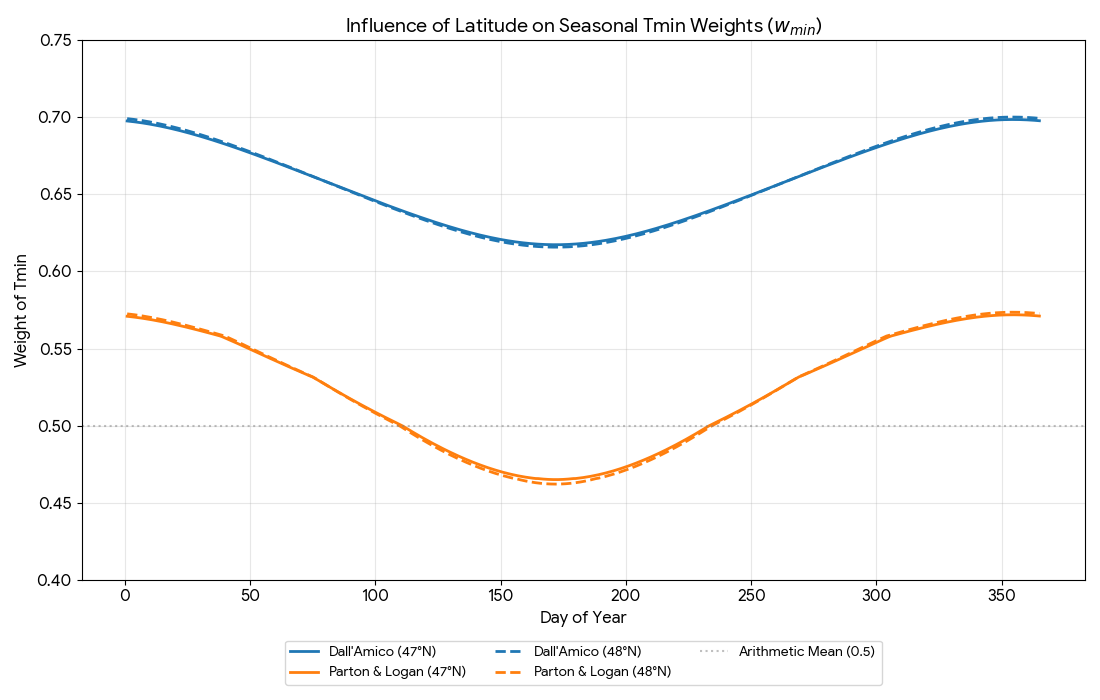
Why this is worth being aware of: Tmean enters the model in several places, so a systematic offset in the input propagates into several processes simultaneously:
- The rain/snow partition uses Tmean against the
SNOWTRT–RAINTRTthresholds — a cooler Tmean shifts more precipitation to snow. - Snowmelt is temperature-index based — a cooler Tmean reduces simulated melt.
- Evapotranspiration (Thornthwaite, when
ETPCONTROL = 0) is driven by Tmean and the long-termTMMON— a cooler Tmean reduces simulated ET.
As a starting point:
| Catchment setting | A reasonable starting choice |
|---|---|
| Alpine, snow-dominated | "dall_amico" |
| Lowland / pre-Alpine, rain-dominated | "simple" (default) or "parton_logan" |
| Mixed or uncertain | Compare methods and inspect simulated snow and ET against observations |
Step 4: Process Potential Evapotranspiration (Optional)
If you want to supply external ETP instead of using COSERO’s internal Thornthwaite calculation, write_winfore_et0() processes the WINFORE daily ET0 product in the same way.
write_winfore_et0(
  nc_dir       = "C:/COSERO/data/GeoSphere/WINFORE_ET0",
  output_dir   = "C:/COSERO/MyCatchment/input",
  model_zones  = zones,
  nz_col       = "NZ",
  years        = 1991:2024,
  write_binary = TRUE,
  n_cores      = 4,
  na_fill      = "mean"
)
To activate external ETP, set ETPCONTROL = 1 in MetDefaults.txt and point ETPFILE to the generated file. Otherwise leave ETPCONTROL = 0 and COSERO estimates ETP internally from the TMMON parameter (mean monthly zone temperature).
NoteBinary meteorological input files
The functions to process the meteorological data also support the output of binary files, by defining write_binary = TRUE. Binary files have the advantage of speeding up the reading of inputs during modelling, but have the disadvantage of being a “black box”, since you can not open the files with a text editor to check the content.
Part 3: Model Input Files — Met Forcing, Discharge & Defaults
MetDefaults.txt
The MetDefaults.txt file in the project root tells COSERO which input files to read and how ETP is handled:
### USER action necessary below ###
ASCIIorBIN (define, if datafiles are ASCII (0) or Binary (1))
0
PRECFILE (input precipitation file, read from directory "/input")
P_NZ_1991-2024.txt
TEMPFILE (input temperature file, read from directory "/input")
T_NZ_1991-2024.txt

ETPCONTROL (how ETP is calculated; 0 = Thornthwaite, 1 = external file)
0
ETPFILE (input ETP file; relevant if ETPCONTROL=1)
ETP_NZ_1991-2024.txt| Setting | Values | Description |
|---|---|---|
ASCIIorBIN |
0 / 1 | File format: 0 = ASCII text, 1 = Binary |
PRECFILE |
filename | Precipitation input file |
TEMPFILE |
filename | Temperature input file |
ETPCONTROL |
0 / 1 | ETP source: 0 = Thornthwaite internal, 1 = external file |
ETPFILE |
filename | ETP input file (only used if ETPCONTROL = 1) |
Meteorological Input File Format
All three meteorological files (precipitation, temperature, ETP) share the same structure. The CoseRo functions generate these files automatically; the description below is for reference and manual inspection. It is valid for the ASCII outputs (e.g. P_NZ_1991-2024.txt).
ImportantFile Format Requirements
- No header row
- One row per time step
- Space-separated values
- No missing values (NA) or gaps
- Precipitation must be non-negative
Column structure:
YYYY MM DD hh mm value_NZ1 value_NZ2 value_NZ3 ...| Column | Content | Example |
|---|---|---|
| 1 | Year (YYYY) | 2003 |
| 2 | Month (MM) | 01 |
| 3 | Day (DD) | 15 |
| 4 | Hour (hh) | 00 |
| 5 | Minute (mm) | 00 |
| 6+ | Values for each zone NZ = 1, 2, 3, … | 0.5 0.8 0.6 … |
Example — daily precipitation file (8 zones):
2003 01 01 00 00 0.103 0.110 0.115 0.113 0.128 0.132 0.165 0.144
2003 01 02 00 00 0.150 0.152 0.153 0.147 0.145 0.158 0.110 0.090
2003 01 03 00 00 0.050 0.089 0.166 0.118 0.127 0.175 0.151 0.140
...
Example — daily temperature file (8 zones):
2003 01 01 00 00 -4.600 -4.559 -5.066 -4.706 -4.707 -5.215 -4.951 -4.652
2003 01 02 00 00 -4.800 -4.750 -5.322 -5.041 -4.963 -5.529 -5.230 -4.918
2003 01 03 00 00 -3.100 -3.020 -3.811 -3.512 -3.440 -4.010 -3.710 -3.380
...
Discharge Observations (Qobs)
Observed discharge is needed for model calibration and validation. write_ehyd_qobs() reads raw eHYD daily discharge CSV files (Q-Tagesmittel-*.csv, downloaded from eHYD) and writes the COSERO QOBS file. You provide a mapping from eHYD gauge IDs (HZB-Nummer) to COSERO subbasin IDs (NB).
library(CoseRo)

# Map eHYD HZB-Nummer to COSERO subbasin IDs (NB)
# Wildalpen example: 3 gauges, upstream-to-downstream
gauge_mapping <- c(
  "210864" = 1,   # Gußwerk / Salza      → NB 1
  "210880" = 2,   # Weichselboden        → NB 2
  "210898" = 3    # Wildalpen / Salza    → NB 3
  # "NA"   = 4   # uncomment for an ungauged subbasin — see callout
)

write_ehyd_qobs(
  input_dir      = "C:/COSERO/data/eHYD/raw",    # folder with Q-Tagesmittel-*.csv
  output_file    = "C:/COSERO/MyCatchment/input/Qobs.txt",
  gauge_to_nb    = gauge_mapping,
  catchment_name = "COSERO-Wildalpen",
  start_date     = "1991-01-01",
  end_date       = "2024-12-31"
)
Tip
The HZB-Nummer for each gauge is found in the eHYD filename (e.g. Q-Tagesmittel-210864.csv), the metadata in each file, and in the eHAO shapefile gauging station attribute table (hzbnr field). Missing discharge values are written as -0.01 by default, which COSERO recognises as a gap.
Ungauged subbasins: declare them in gauge_to_nb with a sentinel key ("NA", "-999", or any negative numeric string). All days for that subbasin are then filled with -999 — a permanent no-gauge flag, distinct from na_value = -0.01 which marks temporarily missing days. Repeat the sentinel for multiple ungauged subbasins, e.g. c("210864" = 1, "NA" = 2, "NA" = 3).
The defaults.txt Configuration File
defaults.txt is the central configuration file for a COSERO project. It tells the model where to find its input files, what the simulation period is, and how much output to produce. It lives in the input/ folder of your project and is read every time COSERO runs.
A typical defaults.txt for the Wildalpen case study looks like this:
This file contains default settings for COSERO

PROJECTINFO (default project info, written into first line of each output file)
COSERO Wildalpen

DATAFILE (default input data file containing observed discharge, read in from directory "input")
Qobs.txt

PARAFILE (default input parameter file, read in from directory "input")
para_ini.txt

IKL (# of snow classes)
5

NCLASS (# of Landuse classes)
10

STARTDATE (start date of simulation period in format yyyy mm dd hh mm)
1991 1 1 0 0

ENDDATE (end date of simulation period in format yyyy mm dd hh mm)
2024 12 31 0 0

SPINUP (length of spin-up period without evaluation [time-steps])
365

OUTPUTTYPE (Sets the output evaluation extent: 1 - only QSIM; 2 - ZRVIEW compatible; 3 - full evaluation)
1

SC_FLAG (Use local subbasin area (EZFL_B, "0") or total upstream catchment area (EZFL_T, "1") for runoff depth / flux calculations)
1

OUTCONTROL (if set to "1", zonal values will be written for every time step: folder cdr/output is needed; very slow; outputtype must be "3"; otherwise set to "0")
0

RUNOFFFILE (default output file for simulated runoff of a single run, written to directory "output")
COSERO.runoff

STATSFILE (default output file for performance statistics of a single run, written to directory "output")
statistics.txt

OPTFILE (default output file for progress of optimization, written to directory "output")
optprogress.txt

ADDFLUXCONT (if set to "1", file Qadd with additional inflow from outside the study area is read in; otherwise set to "0")
0

ADDFLUXFILE (additional inflow in m³/s added to specified subbasins/zones. Starts with an NB-TONZ mapping header, followed by the time series. Read in from directory "input")
Qadd.txt

ADDREGCONT (if set to "1", file Qreg with regression parameters for estimating inflow from outside the study area is read in; otherwise set to "0")
0

ADDREGFILE (regression parameters (up to 3 predictors) to calculate subbasin inflow based on discharge in other (predictor) subbasins. Read in from directory "input")
reg_para.txt

WRITERASTERS (write state/flux-rasters for use in FEWS)
raster_write.txt

BINDATAFILE (default input binary data file, read in from directory "cdr/input", not used)
not_used.dat
The settings you will need to adjust for your own catchment are:
defaults.txt settings
| Setting | Description | Typical value |
|---|---|---|
PROJECTINFO |
Label written into every output file header | Your catchment name |
DATAFILE |
Observed discharge file (Qobs) | Qobs.txt |
PARAFILE |
Parameter file to use for the run | para_ini.txt |
STARTDATE / ENDDATE |
Simulation period (yyyy mm dd hh mm) | Match your data record |
SPINUP |
Warm-up period in time steps (daily → days) | 365 |
OUTPUTTYPE |
Output extent: 1 = discharge only, 3 = full outputs | 3 for Module 3 & 4 |
SC_FLAG |
Runoff depth basis: 0 = local zone area, 1 = total upstream area | 1 (recommended) |
In practice, the CoseRo package manages defaults.txt transparently — functions like run_cosero(), optimize_cosero_dds(), and the Shiny app read and update the file automatically so you rarely need to edit it by hand. Understanding its structure is nonetheless useful: when something unexpected happens (wrong simulation period, missing output files, a run that is slower than expected), defaults.txt is the first place to look.
The easiest way to start is to copy defaults.txt from the Wildalpen example project and adjust the settings for your own catchment. You can inspect the current settings at any time with:
library(CoseRo)

show_cosero_defaults(project_path)   # prints all settings to console
defaults <- read_defaults(project_path)  # returns a named list for programmatic access
ImportantRequired: Copy Auxiliary Files from the Example Project
Your workflow will generate the core input files (meteorological inputs, para_ini.txt, Qobs.txt). However, several auxiliary files (inclduing defaults.txt) are not generated by the workflow above and must be copied manually from the example project into your own input/ folder:
| File | Purpose |
|---|---|
defaults.par |
Central configuration file |
radmat.par |
Radiation parameters required for glacier module |
raster_write.txt |
Spatial output configuration |
Qadd_example.txt |
Template for additional discharge inputs (adapt if needed) |
reg_para_example.txt |
Template for regression parameter settings |
Copy these from C:/COSERO/Wildalpen/input/ to your own project’s input/ folder before running the model.
What You Should Know
After completing this module you should understand the following concepts and be able to reproduce the corresponding steps for your own catchment. These points may also serve as a guide for your presentation.
- Project structure: Explain the COSERO folder and file structure. Set up a new project directory using
setup_cosero_project()and verify all required files are present withshow_required_files(). - Spatial discretization: Describe the role of subbasins and zones in COSERO. Explain why zones are the basic modelling unit and how they relate to the spatial patterns of landscape attributes (soil, vegetation, elevation). Produce aggregated catchment polygons with correct NB ordering and routing. Understand, how the COSERO zone generation workflow works (starting in QGIS to applying R)
- Initial parameter file: Explain how the a priori parameter file is derived from raster maps of landscape attributes and what assumptions are embedded in this step.
- Meteorological input processing: Download SPARTACUS and WINFORE data and convert them to COSERO binary input format using
write_spartacus_precip(),write_spartacus_temp(), andwrite_winfore_et0(). Describe the temporal shift correction and explain why it is needed. - Precipitation undercatch: Explain what precipitation undercatch is, why it matters in alpine catchments, and how the
PCORparameter is used to compensate for it. - Discharge observations: Convert eHYD gauge data to COSERO QOBS format using
write_ehyd_qobs(). Verify that gauge IDs are correctly mapped to subbasin NB numbers and that the time series covers the intended simulation period. - Input file completeness: Use
show_required_files()to confirm that all mandatory files are present before attempting a first model run in Module 3.
Document created: 2026-05-22
References
European Space Agency: Copernicus Global Digital Elevation Model, https://doi.org/10.5069/G9028PQB, 2024.
Feigl, M., Herrnegger, M., and Schulz, K.: Distilling hydrological and land-surface model parameters from physio-geographical properties using text-generating AI, Nature Water, 4, 158–168, https://doi.org/10.1038/s44221-026-00583-3, 2026.
Gemeinderatsausschuß der Stadt Wien: Die Zweite Kaiser-Franz-Josef-Hochquellenleitung der Stadt Wien: Eine Gedenkschrift, Stadt Wien, 1910.
Gupta, H. V.: Deep learning can facilitate physically interpretable geoscientific modelling, Nature Water, 4, 118–119, https://doi.org/10.1038/s44221-026-00589-x, 2026.
Haberl, U.: Konzeptionelle Schneemodellierung in einem hydrologischen Modell: Ansätze und Analysen zur räumlichen Verteilung von Parametern der Prozesse Akkumulation, Verteilung und Schmelze, Dissertation, Universität für Bodenkultur Wien, Wien, 2021.
Herrnegger, M., Nachtnebel, H. P., and Schulz, K.: From runoff to rainfall: inverse rainfall–runoff modelling in a high temporal resolution, Hydrology and Earth System Sciences, 19, 4619–4639, https://doi.org/10.5194/hess-19-4619-2015, 2015.
Herrnegger, M., Senoner, T., and Nachtnebel, H. P.: Adjustment of spatio-temporal precipitation patterns in a high Alpine environment, Journal of Hydrology, 556, 913–921, https://doi.org/10.1016/j.jhydrol.2016.04.068, 2018.
Koblizek, R. and Süssenbek, N.: Die Trinkwasserversorgung der Stadt Wien von ihren Anfängen bis zur Gegenwart, Wien, 1999--2000.
Koppensteiner, S. J. and Plan, L.: Anspringverhalten der Tagwässer der Kläfferquellen (Hochschwab, Steiermark), Die Höhle, 70, 2019.
Maier, P., Ehrendorfer, C., Lücking, S., Pulka, T., Lehner, F., Herrnegger, M., Formayer, H., and Koch, F.: Undercatch corrected gridded precipitation data to improve hydrological modeling in high-alpine orography, EGUsphere, 2026, 1–35, https://doi.org/10.5194/egusphere-2025-6382, 2026.
Plan, L., Kuschnig, G., and Stadler, H.: Chapter 10.2 - case study: Kläffer spring—the major spring of the vienna water supply (austria), in: Groundwater hydrology of springs, edited by: Kresic, N. and Stevanovic, Z., Butterworth-Heinemann, Boston, 411–427, https://doi.org/10.1016/B978-1-85617-502-9.00020-7, 2010.
Pulka, T., Herrnegger, M., Ehrendorfer, C., Lücking, S., Avanzi, F., Formayer, H., Schulz, K., and Koch, F.: Evaluating precipitation corrections to enhance high-alpine hydrological modeling, Journal of Hydrology, 645, 132202, https://doi.org/10.1016/j.jhydrol.2024.132202, 2024.
Pulka, T., Ehrendorfer, C., Lievens, H., Koch, F., Schulz, K., Formayer, H., Avanzi, F., Girotto, M., and Herrnegger, M.: Assimilation of Sentinel-1 C-band SAR snow depth retrievals in operational hydrological modeling of high-alpine catchments, https://doi.org/10.2139/ssrn.6215391, 2025.
Stadt Wien - Wiener Wasser: Trinkwasserversorgung und Quellenschutz: Der Weg des Wassers, Magistrat der Stadt Wien, MA 31, 2023.
Wiener Wasser: Zahlen, Daten, Fakten: https://www.wien.gv.at/wienwasser/versorgung/statistik.html, last access: 29 December 2025.
Zweite Hochquellenleitung: https://www.geschichtewiki.wien.gv.at/Zweite_Hochquellenleitung, last access: 29 December 2025.
Zeitfogel, H., Herrnegger, M., and Schulz, K.: Regional-scale assessment of groundwater recharge and the water balance for Austria (Version 1.0), https://doi.org/10.5281/zenodo.13752163, 2024.
Zeitfogel, H., Herrnegger, M., and Schulz, K.: Regional-Scale Assessment of Groundwater Recharge and the Water Balance for Austria, Journal of Hydrology: Regional Studies, 59, 102297, https://doi.org/https://doi.org/10.1016/j.ejrh.2025.102297, 2025.