library(CoseRo)
library(ggplot2)
library(dplyr)
library(tidyr)

project_path <- "C:/COSERO/MyCatchment"   # adjust to your project
subbasins    <- c("001", "002", "003")     # adjust to your catchment

base_settings <- list(
  STARTDATE  = "2010 1 1 0 0",
  ENDDATE    = "2020 12 31 0 0",
  SPINUP     = 365,
  OUTPUTTYPE = 1,
  PARAFILE   = "para_ini.txt"
)

# Run COSERO with initial parameters
result_base <- run_cosero(
  project_path      = project_path,
  defaults_settings = base_settings,
  statevar_source   = 1   # cold start
)

# Check performance for each subbasin
for (sb in subbasins) {
  nse <- extract_run_metrics(result_base, sb, "NSE")
  kge <- extract_run_metrics(result_base, sb, "KGE")
  cat(sprintf("Subbasin %s:  NSE = %.3f  |  KGE = %.3f\n", sb, nse, kge))
}Mathew Herrnegger · mathew.herrnegger@boku.ac.at
Institute of Hydrology and Water Management (HyWa) BOKU University Vienna, Austria
LAWI301236 · Distributed Hydrological Modeling with COSERO
![]()
Introduction
In Module 2 you built a spatially distributed COSERO model: subbasins, zones, meteorological inputs, and an initial parameter file derived from landscape attributes. This module picks up from there. The a priori parameters are a reasonable starting point, but they are unlikely to produce good discharge simulations right away — the gap between landscape maps and effective model parameters may be too large.
This module covers three steps to close that gap:
- Running the model and exploring results — using both code and the interactive Shiny app
- Understanding parameter effects — how parameters are modified while preserving spatial patterns
- Sensitivity analysis — a systematic, quantitative answer to the question: which parameters matter?
The next step — automatic calibration — follows in Module 4, informed by the sensitivity results from this module.
NoteA word of caution
Calibration can produce impressive-looking fits. This does not mean the model is “correct” — it means the optimiser found parameter values that minimise the chosen objective function over the calibration period. Different objective functions, different periods, or different spatial resolutions can yield very different parameter sets, all with similar performance. This problem — known as equifinality — is not a bug; it reflects the fundamental under-determination of hydrological models.
A concrete example: if the precipitation input is systematically too low — common in alpine catchments with gauge undercatch — a calibration algorithm will compensate by suppressing evapotranspiration parameters. The resulting water balance may close neatly (\(Q_{sim} \approx Q_{obs}\)), but the model underestimates evapotranspiration and overestimates the fraction of precipitation that becomes runoff. The “good” discharge fit hides a fundamentally wrong partitioning of the water balance. This kind of error is invisible in the objective function but becomes consequential the moment you use the model for anything beyond reproducing the calibration period.
As Kirchner (2006) noted, it is entirely possible to get the “right answers” for the “wrong reasons.” Vít Klemeš (1986) warned against precisely this kind of uncritical modelling practice. Keep this in mind throughout: use the tools in this module not just to maximise a score, but to interrogate whether your model’s internal behaviour remains physically plausible. The chief objective of any modelling exercise is to represent the real world hydrological system in a realistic and plausible way, and to know the deficits and shortcomings present in your model.
Part 1: First Run with Initial Parameters
NoteWhat you’ll learn
Run COSERO with a priori parameters, read performance metrics, and inspect the model configuration — the starting point for everything that follows.
After completing Module 2, your project directory contains all necessary inputs. The first step is to run COSERO with the a priori parameters and see how well (or poorly) the model reproduces observed discharge. When setting up the code, check things like project_path, subbasins or which parameter file (argument PARAFILE) is being used. Adopt these values to your setup.
TipOrganising your script
As you copy code from Modules 3 and 4 into your own R script, use comment hierarchies to keep it navigable. RStudio’s document outline (Ctrl+Shift+O) reads # SECTION #### and ## sub-section #### markers, making it easy to jump between parts. See R Introduction — Comment Hierarchies for the convention used in this course.
Don’t be surprised if the initial NSE is low or even negative. The a priori parameters were derived from maps and transfer functions — they reflect landscape properties at best approximately, and many model parameters (recession constants, percolation rates) have no direct physical observable at the relevant scale.
Inspecting Parameters and Configuration
Before changing anything, understand what the current parameter values are and how the model is configured.
# Show available configuration settings
show_cosero_defaults()

# Read current settings
defaults <- read_defaults(file.path(project_path, "input", "defaults.txt"))
cat("Parameter file:", defaults$PARAFILE, "\n")

# Read parameter values for selected parameters across all zones
par_file <- file.path(project_path, "input", defaults$PARAFILE)
params   <- read_parameter_table(
  par_file,
  param_names = c("BETA", "M", "KBF", "TAB1", "H1", "TVS1"),
  zone_id     = "all"
)
print(params)

# Show the average of the parameters over all zones
colMeans(params[-1]) # we remove the first column, which is NZ_

# See distribution of a parameter, e.g. KBF
hist(params$KBF)

# Read parameter values for ALL parameters across all zones
params_all   <- read_cosero_parameters(par_file)
print(head(params_all))
The output shows one row per zone. The spatial variability across zones reflects the landscape attributes used during parameter generation (Module 2). This variability is something we want to preserve when modifying parameters.
Part 2: Interactive Exploration with the CoseRo Shiny App
NoteWhat you’ll learn
Use the CoseRo Shiny app to interactively explore model results, modify parameters, and build intuition for how COSERO behaves — before writing any analysis code.
The CoseRo package includes a modern, interactive dashboard for running COSERO and exploring results. Launch it with a single command:
launch_cosero_app(project_path)The app opens in your browser and provides different tabs, each focused on a different aspect of model analysis. It supports a dark mode toggle and is built with Bootstrap 5 for a responsive layout.
Tab 1: COSERO Run
The Run tab is the control centre for model execution and parameter management.
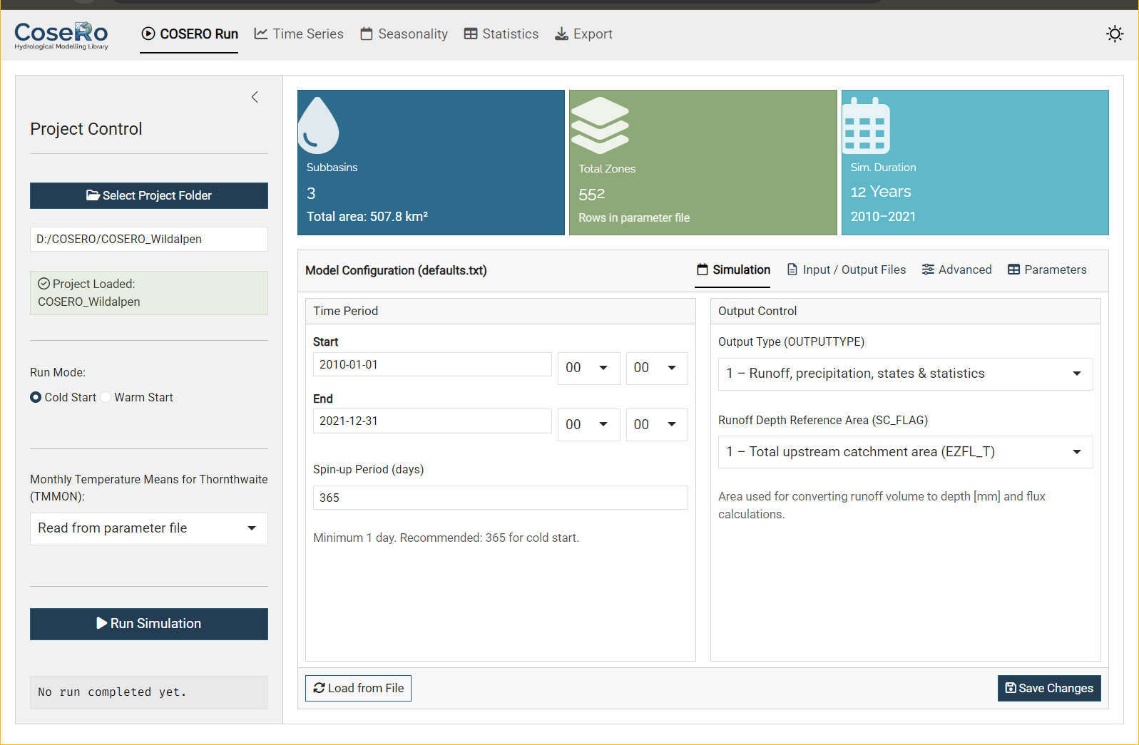
Sidebar: Select your project folder (browse or paste a path), choose cold or warm start, set the TMMON option, and run the simulation.
Value boxes at the top show key project metadata: number of subbasins, total zones, and simulation duration — all read directly from the parameter and configuration files.
Model Configuration — a tabbed editor for defaults.txt:
- Simulation: Start/end date and time, spin-up period, output type (1–3), SC_FLAG
- Input/Output Files: Parameter file (PARAFILE), observation file, output file names
- Advanced: Snow/landuse classes (IKL, NCLASS), zonal output control, boundary conditions
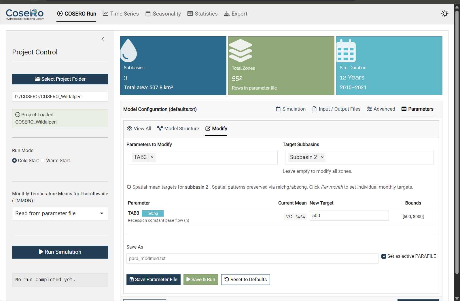
Parameters — three sub-tabs for viewing and modifying the parameter file:
- View All: Read-only table of all zone parameters (sortable, searchable)
- Model Structure: Conceptual COSERO model diagram
- Modify: Interactive spatial-mean target editor — the key feature for hands-on exploration:
- Parameters are grouped by category (Snow, Soil, Runoff, Groundwater, Evapotranspiration, etc.)
- Filter zones by subbasin to inspect and modify specific parts of the catchment
- Set new target values within the bounds defined in
parameter_bounds.csv - Monthly parameters (TCOR, PCOR, TMMON, INTMAX, ETVEGCOR, etc.) support per-month editing in a 4×3 grid (Jan–Dec) or uniform mode
- Three actions: Save Parameter File, Save & Run (modify and immediately execute), Reset to Defaults
TipExplore before you code
Use the Modify tab to experiment: increase soil storage (M), speed up surface flow (TAB1), or add a precipitation correction (PCOR). Hit “Save & Run” and switch to the Time Series tab and load the results to see the effect immediately. This interactive loop builds intuition much faster than writing scripts — but once you know which parameters matter, the code-level approach (Part 3/4) gives you reproducibility and automation.
Tab 2: Time Series
The Time Series tab provides the core diagnostic view.
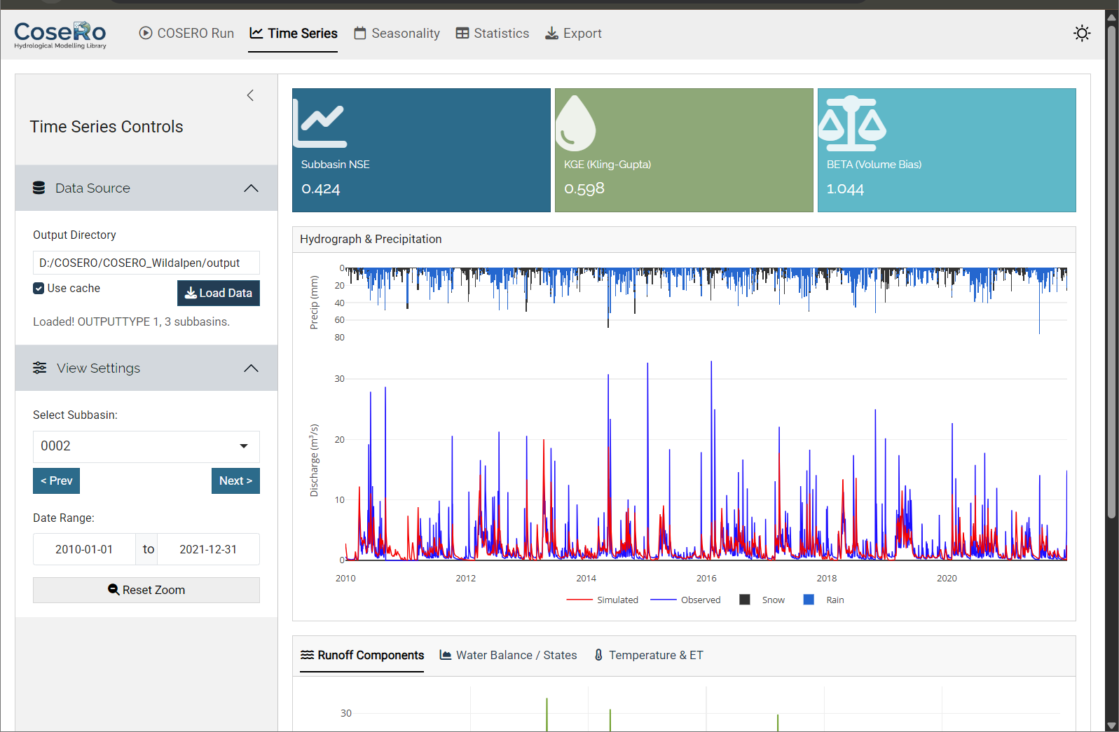
- Combined hydrograph: Inverted precipitation bars (top) and observed vs simulated discharge (bottom) with linked zoom — zoom in on one panel and the other follows
- Runoff components: QAB123 (total), QAB23 (subsurface), QAB3 (baseflow) — stacked or as separate lines
- Water balance states: Soil moisture (BW0), groundwater (BW3), snow water equivalent (SWW)
- Temperature & ET: Temperature line and evapotranspiration (requires OUTPUTTYPE ≥ 2)
- Value boxes: NSE, KGE, and volume bias (BETA) for the selected subbasin
Navigate between subbasins with Previous/Next buttons. Reset zoom to return to the full period.
Tab 3: Seasonality
The Seasonality tab aggregates results to a monthly climatology (Jan–Dec):
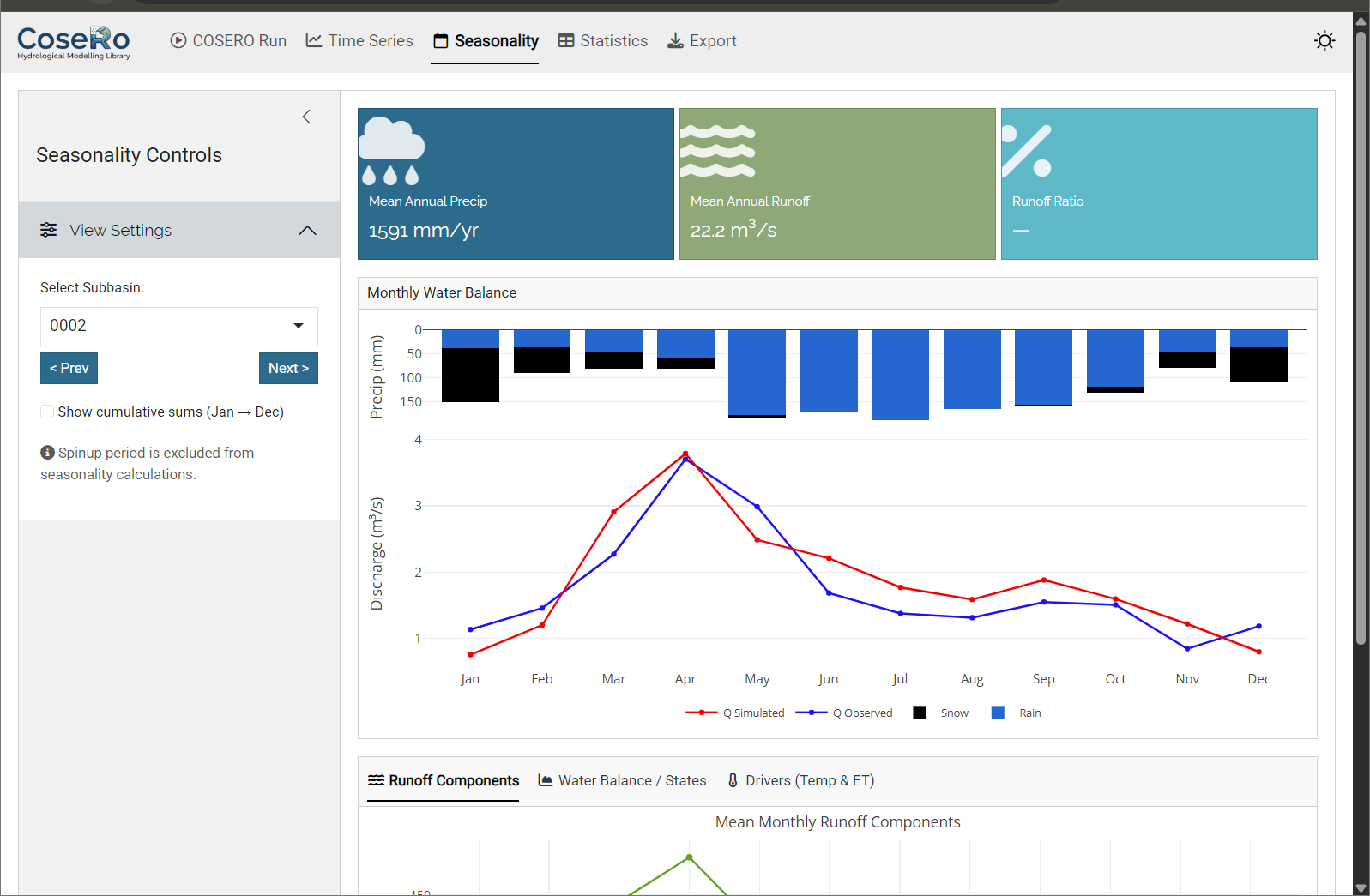
- Monthly regime: inverted precipitation bars + observed/simulated discharge
- Monthly runoff components and water balance breakdown
- Cumulative sums toggle for tracking annual accumulation
- Value boxes: seasonal NSE, mean annual precipitation, runoff ratio
Tab 4: Model Performance
The Performance tab provides a cross-subbasin comparison:
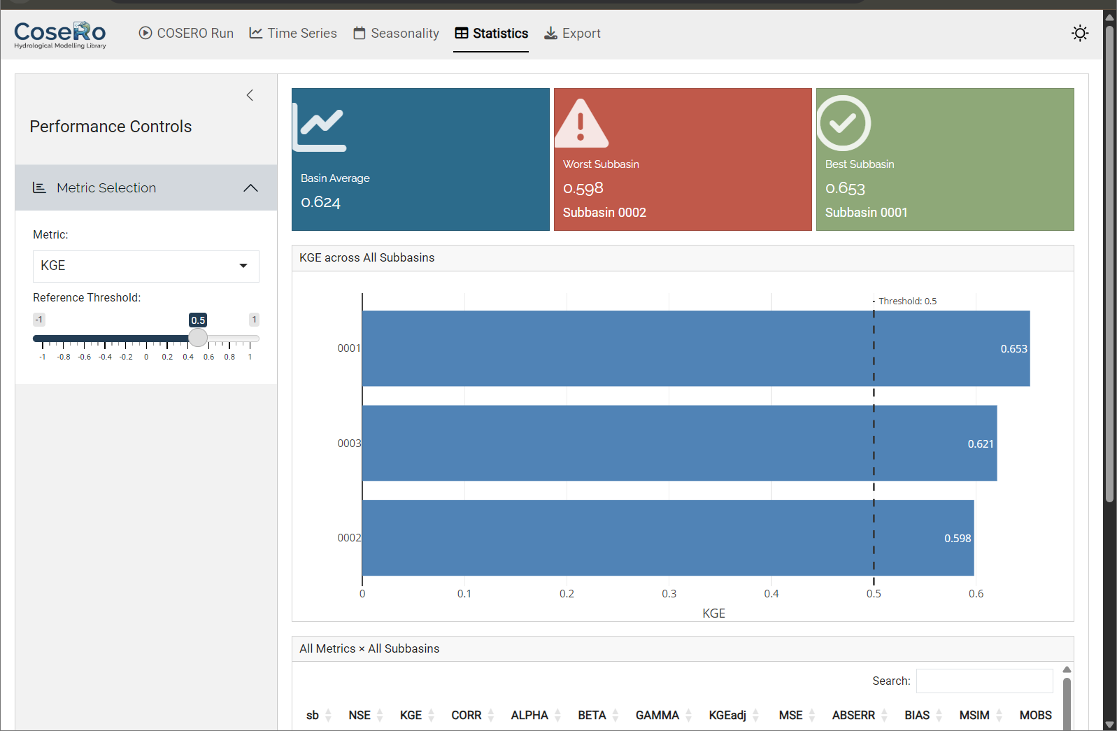
- Select a metric (NSE, KGE, KGEadj, BETA) and set a “good performance” threshold
- Horizontal bar chart: all subbasins ranked by the selected metric, colour-coded by threshold
- Summary table with conditional formatting
- Value boxes: network average, worst-performing subbasin, percentage above threshold
Tab 5: Export
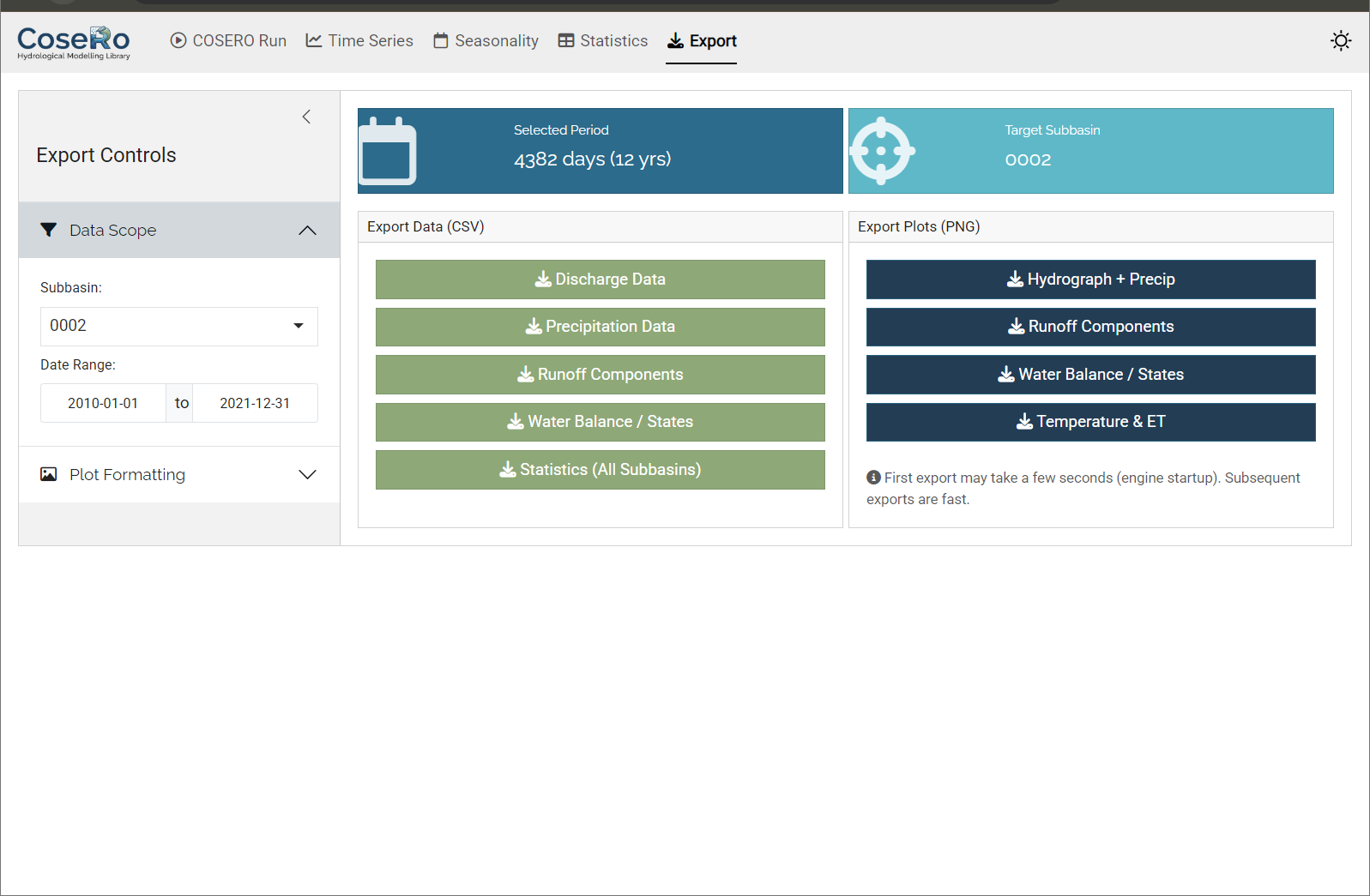
- Download CSV files (discharge, components, water balance per subbasin)
- Export high-resolution PNG images of all diagnostic plots
- Filter by subbasin and date range before exporting
Part 3: Performance Metrics
NoteWhat you’ll learn
Understand how NSE and KGE quantify model performance — and why no single number tells the full story.
Before discussing parameter modification and sensitivity analysis, we need to define what “good” means. Performance metrics quantify the agreement between simulated and observed discharge. No single metric captures all aspects of hydrological behaviour, and each has known biases.
Nash-Sutcliffe Efficiency (NSE)
The Nash-Sutcliffe Efficiency (Nash and Sutcliffe, 1970) is perhaps the most widely used metric in hydrology:
\[ \text{NSE} = 1 - \frac{\sum (Q_{obs,t} - Q_{sim,t})^2}{\sum (Q_{obs,t} - \overline{Q_{obs}})^2} \]
- NSE = 1: perfect match
- NSE = 0: the model is as good as the mean of observations
- NSE < 0: worse than the mean
NSE is dominated by high flows because it uses squared errors. A model can have a high NSE while systematically misrepresenting low flows.
Kling-Gupta Efficiency (KGE)
Gupta et al. (2009) showed that NSE implicitly conflates correlation, bias, and variability in ways that are difficult to interpret. They proposed the Kling-Gupta Efficiency, which separates these components explicitly:
\[ \text{KGE} = 1 - \sqrt{(r - 1)^2 + (\alpha - 1)^2 + (\beta - 1)^2} \]
where \(r\) = correlation, \(\alpha\) = variability ratio (\(\sigma_{sim} / \sigma_{obs}\)), and \(\beta\) = bias ratio (\(\overline{Q_{sim}} / \overline{Q_{obs}}\)). KGE decomposes performance into three interpretable components: timing, variability, and volume. Values above 0 are generally considered informative, though this depends on the application (Knoben et al., 2019).
Volume Bias (BETA)
The bias ratio \(\beta\) — one of the three KGE components — deserves special attention because it directly quantifies the water balance closure:
\[ \beta = \frac{\overline{Q_{sim}}}{\overline{Q_{obs}}} \]
- \(\beta\) = 1: no systematic bias — the model produces the correct total volume
- \(\beta\) > 1: the model overestimates discharge (too much water leaves the catchment)
- \(\beta\) < 1: the model underestimates discharge (water is “lost” — likely to excessive ET or storage)
Unlike NSE and KGE, which aggregate timing, variability, and volume into a single number, \(\beta\) isolates the volume question: does the model get the overall water balance right? This is critical because a model can achieve a high NSE or KGE while being systematically biased — for example, consistently underestimating baseflow but compensating with overestimated peaks. Such compensation may produce an acceptable overall score but indicates a flawed internal partitioning of the water budget.
In practice, \(\beta\) is the first thing to check. If \(\beta\) deviates substantially from 1, the model’s water balance is wrong regardless of how well the hydrograph shape matches. Common causes include biased precipitation input (gauge undercatch), incorrect evapotranspiration parameterisation, or missing processes (e.g., groundwater losses, inter-basin transfers).
Performance Rating Guidelines
The following tables provide commonly used thresholds for interpreting metric values. These ratings are subjective and context-dependent — a “good” NSE for a data-sparse tropical catchment may be different from what is expected for a well-gauged Alpine basin — but they offer a useful starting point.
NSE Performance Ratings:
| NSE Range | Performance Rating |
|---|---|
| > 0.8 | Excellent |
| 0.6 – 0.8 | Very Good |
| 0.4 – 0.6 | Good |
| 0.2 – 0.4 | Poor |
| ≤ 0.2 | Very Poor |
| < 0 | Unacceptable (worse than mean observation) |
KGE Performance Ratings:
| KGE Range | Performance Rating |
|---|---|
| > 0.9 | Excellent |
| 0.75 – 0.9 | Very Good |
| 0.5 – 0.75 | Good |
| 0 – 0.5 | Poor |
| < 0 | Very Poor |
BETA (Volume Bias) Ratings:
| BETA Range | Performance Rating | Interpretation |
|---|---|---|
| 0.95 – 1.05 | Excellent | Nearly unbiased |
| 0.85 – 0.95 or 1.05 – 1.15 | Good | Slight bias |
| 0.70 – 0.85 or 1.15 – 1.30 | Poor | Significant bias |
| < 0.70 or > 1.30 | Very Poor | Severe bias |
Which Metric to Use?
There is no universally “best” metric. NSE and KGE measure different things and can lead to different calibrated parameter sets. In practice, using multiple metrics provides a more balanced assessment.
ImportantMetrics are summaries, not truths
A single number cannot capture the full range of hydrological behaviour — peak timing, baseflow recession, snow dynamics, seasonal patterns. Always inspect hydrographs and flow duration curves alongside metrics. A model with NSE = 0.8 may still have systematic problems that matter for your application.
Part 4: Parameter Modification
NoteWhat you’ll learn
Modify parameters programmatically while preserving spatial patterns, compare scenarios systematically, and understand the difference between relative and absolute change strategies.
The Shiny app (Part 2) lets you modify parameters interactively. For reproducible, scriptable workflows — especially when comparing multiple scenarios — the code-level approach is essential.
How Parameter Modification Works
A distributed model has parameter values at every zone. When we say “set BETA to 6”, we don’t mean overwriting all zones with the same value — that would destroy the spatial pattern derived from soil maps, land use, and topography. Instead, the CoseRo package uses a spatial-mean targeting strategy.
modify_parameter_table() supports two modification types (defined in parameter_bounds.csv):
Relative change (relchg) — used for most parameters (BETA, M, TAB1, KBF, …):
\[ \text{factor} = \frac{\text{target value}}{\text{spatial mean of original values}} \] \[ \text{new}_i = \text{original}_i \times \text{factor} \]
The ratios between zones are preserved. Example: 3 zones with BETA = [3, 4.5, 6], spatial mean = 4.5. Target = 6 → factor = 1.333 → result: [4.0, 6.0, 8.0].
Absolute change (abschg) — used for temperature-related parameters (TCOR, THRT, RAINTRT, SNOWTRT, TVAR):
\[ \text{offset} = \text{target value} - \text{spatial mean of original values} \] \[ \text{new}_i = \text{original}_i + \text{offset} \]
Absolute differences between zones are preserved.
# Load bounds (contains modification_type for each parameter)
par_bounds <- load_parameter_bounds(parameters = c("BETA", "M", "KBF", "TAB1", "H1", "TVS1"))

# Read original values
original_values <- read_parameter_table(par_file, par_bounds$parameter, zone_id = "all")

# Create a copy and modify — original file is never touched
par_file_mod <- file.path(project_path, "input", "para_mod.txt")
file.copy(par_file, par_file_mod, overwrite = TRUE)

# Set new target spatial means (arbitrary here; check current means with colMeans(original_values[-1]))
new_params <- list(BETA = 6.0, M = 150, KBF = 5000, TAB1 = 10, H1 = 5, TVS1 = 50)
modify_parameter_table(par_file_mod, new_params, par_bounds, original_values,
                       add_timestamp = TRUE)

# Verify
modified_values <- read_parameter_table(par_file_mod, par_bounds$parameter, zone_id = "all")
print(modified_values)

# Run with modified parameters
result_mod <- run_cosero(
  project_path      = project_path,
  defaults_settings = modifyList(base_settings, list(PARAFILE = "para_mod.txt")),
  statevar_source   = 1
)
TipModifying only specific subbasins
By default, all zones are modified. To change parameters only in specific subbasins, use the zones argument together with get_zones_for_subbasins():
zone_map <- get_zones_for_subbasins(project_path, subbasins = "003")
modify_parameter_table(par_file_mod, new_params, par_bounds, original_values,
                       zones = zone_map$zones)
Comparing Parameter Scenarios
Rather than guessing individual parameter values, define a set of physically motivated scenarios and compare their effects. Each scenario starts fresh from the original parameter file — modifications are never stacked.
scenarios <- list(
  "base"           = NULL,                                    # no modification
  "low_storage"    = list(M = 100),                           # less soil storage
  "fast_response"  = list(TAB1 = 5, H1 = 1, TVS1 = 20),       # faster surface flow
  "precip_plus20"  = list(PCOR = 1.2)                         # +20% precipitation
)

scenario_params <- c("BETA", "M", "TAB1", "H1", "TVS1", "PCOR")
par_bounds_all  <- load_parameter_bounds(parameters = scenario_params)
orig_vals       <- read_parameter_table(par_file, scenario_params, zone_id = "all")

scenario_results <- list()
scenario_metrics <- data.frame()

for (name in names(scenarios)) {
  if (is.null(scenarios[[name]])) {
    settings <- base_settings
  } else {
    tmp <- file.path(project_path, "input", paste0("para_", name, ".txt"))
    file.copy(par_file, tmp, overwrite = TRUE)
    modify_parameter_table(tmp, scenarios[[name]], par_bounds_all, orig_vals)
    settings <- modifyList(base_settings, list(PARAFILE = paste0("para_", name, ".txt")))
  }

  res <- run_cosero(project_path, defaults_settings = settings,
                    statevar_source = 1, quiet = TRUE)
  scenario_results[[name]] <- res

  for (sb in subbasins) {
    scenario_metrics <- rbind(scenario_metrics, data.frame(
      scenario = name, subbasin = sb,
      NSE = extract_run_metrics(res, sb, "NSE"),
      KGE = extract_run_metrics(res, sb, "KGE"),
      BETA = extract_run_metrics(res, sb, "BETA")
    ))
  }
}

# Restore defaults.txt to the original parameter file
modify_defaults(
  defaults_file = file.path(project_path, "input", "defaults.txt"),
  settings = base_settings,
  quiet = TRUE
)

# View results
print(scenario_metrics)
The precip_plus20 scenario is worth particular attention. Precipitation is the main driver of the water balance, yet it is also one of the most uncertain inputs — especially in alpine terrain with sparse gauge networks and systematic undercatch of snowfall. If this scenario improves performance substantially, it suggests that input uncertainty may matter more than parameter uncertainty.
Diagnostic Plots
Metrics alone don’t tell the full story. Visual comparison reveals where and how simulations differ.
Show/hide: Scenario comparison plots
library(ggplot2)
library(dplyr)
library(tidyr)

plot_dir <- file.path(project_path, "single_run_results")
dir.create(plot_dir, showWarnings = FALSE, recursive = TRUE)

# --- Bar chart: all scenarios ---
metrics_long <- scenario_metrics |>
  pivot_longer(cols = c(NSE, KGE), names_to = "metric", values_to = "value")

p_scenario <- ggplot(metrics_long, aes(x = scenario, y = value, fill = metric)) +
  geom_col(position = position_dodge(width = 0.7), width = 0.6) +
  facet_wrap(~subbasin, labeller = labeller(
    subbasin = function(x) paste("Subbasin", x))) +
  geom_hline(yintercept = 0, color = "grey40") +
  scale_fill_manual(values = c(NSE = "#2166ac", KGE = "#b2182b")) +
  labs(title = "Model Performance Across Parameter Scenarios",
       x = NULL, y = "Metric Value", fill = NULL) +
  theme_bw() +
  theme(axis.text.x = element_text(angle = 35, hjust = 1), legend.position = "top")
print(p_scenario)
ggsave(file.path(plot_dir, "scenario_performance.png"),
       p_scenario, width = 12, height = 6, dpi = 150)

# --- Hydrograph comparison: baseline vs one scenario ---
compare  <- "fast_response"   # change to explore other scenarios, e.g. low_storage, fast_response or precip_plus20
sb_plot  <- subbasins[length(subbasins)]
sb_id    <- sprintf("%04d", as.numeric(sb_plot))
qobs_col <- paste0("QOBS_", sb_id)
qsim_col <- paste0("QSIM_", sb_id)
spinup   <- 365
idx      <- (spinup + 1):nrow(scenario_results[["base"]]$output_data$runoff)

runoff_base <- scenario_results[["base"]]$output_data$runoff
runoff_scen <- scenario_results[[compare]]$output_data$runoff

nse_base <- extract_run_metrics(scenario_results[["base"]], sb_plot, "NSE")
nse_scen <- extract_run_metrics(scenario_results[[compare]], sb_plot, "NSE")

hydro_df <- data.frame(
  date     = runoff_base$DateTime[idx],
  Observed = runoff_base[[qobs_col]][idx],
  Baseline = runoff_base[[qsim_col]][idx],
  Scenario = runoff_scen[[qsim_col]][idx]
) |> pivot_longer(-date, names_to = "series", values_to = "Q")

hydro_df$series <- factor(hydro_df$series,
                           levels = c("Observed", "Baseline", "Scenario"),
                           labels = c("Observed", "Baseline", compare))

p_hydro <- ggplot(hydro_df, aes(x = date, y = Q, colour = series)) +
  geom_line(aes(linewidth = series, alpha = series)) +
  scale_colour_manual(values = setNames(c("black", "#2166ac", "#d6604d"),
                                         c("Observed", "Baseline", compare))) +
  scale_linewidth_manual(values = setNames(c(0.6, 0.4, 0.3),
                                            c("Observed", "Baseline", compare))) +
  scale_alpha_manual(values = setNames(c(1, 0.8, 0.8),
                                        c("Observed", "Baseline", compare))) +
  labs(title = paste("Hydrograph — Subbasin", sb_plot),
       subtitle = sprintf("Baseline NSE=%.3f  |  '%s' NSE=%.3f",
                           nse_base, compare, nse_scen),
       x = NULL, y = expression(Q~"["*m^3/s*"]"), colour = NULL) +
  theme_bw() + theme(legend.position = "top") +
  guides(linewidth = "none", alpha = "none")
print(p_hydro)
ggsave(file.path(plot_dir, paste0("hydrograph_NB", sb_plot, "_", compare, ".png")),
       p_hydro, width = 14, height = 6, dpi = 150)
Look at the hydrograph critically: Does the scenario shift the timing of peaks? Does it affect baseflow levels? Does it improve one season while degrading another? These patterns tell you more about model behaviour than the aggregate metrics.
The following figures show example outputs for the Wildalpen catchment.
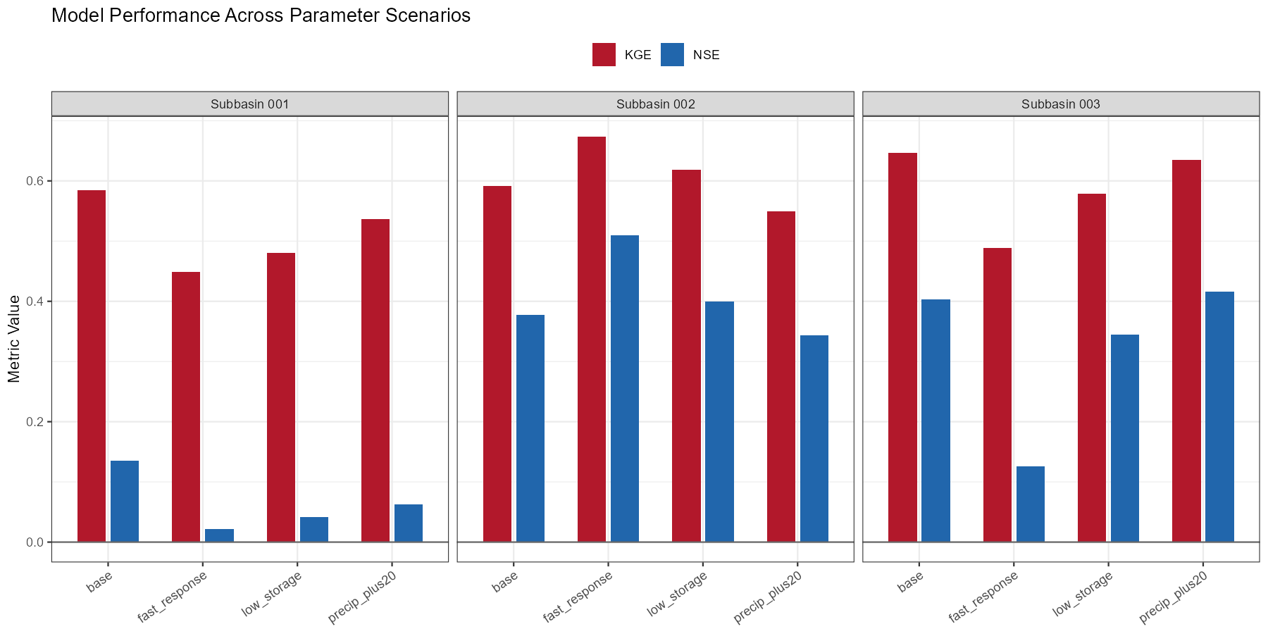
precip_plus20 scenario (+20% precipitation correction) yields the largest improvement, particularly at the outlet (subbasin 003), suggesting that input uncertainty is a dominant factor at this alpine site. The fast_response scenario improves peak timing slightly but degrades volume balance in the upper subbasins.
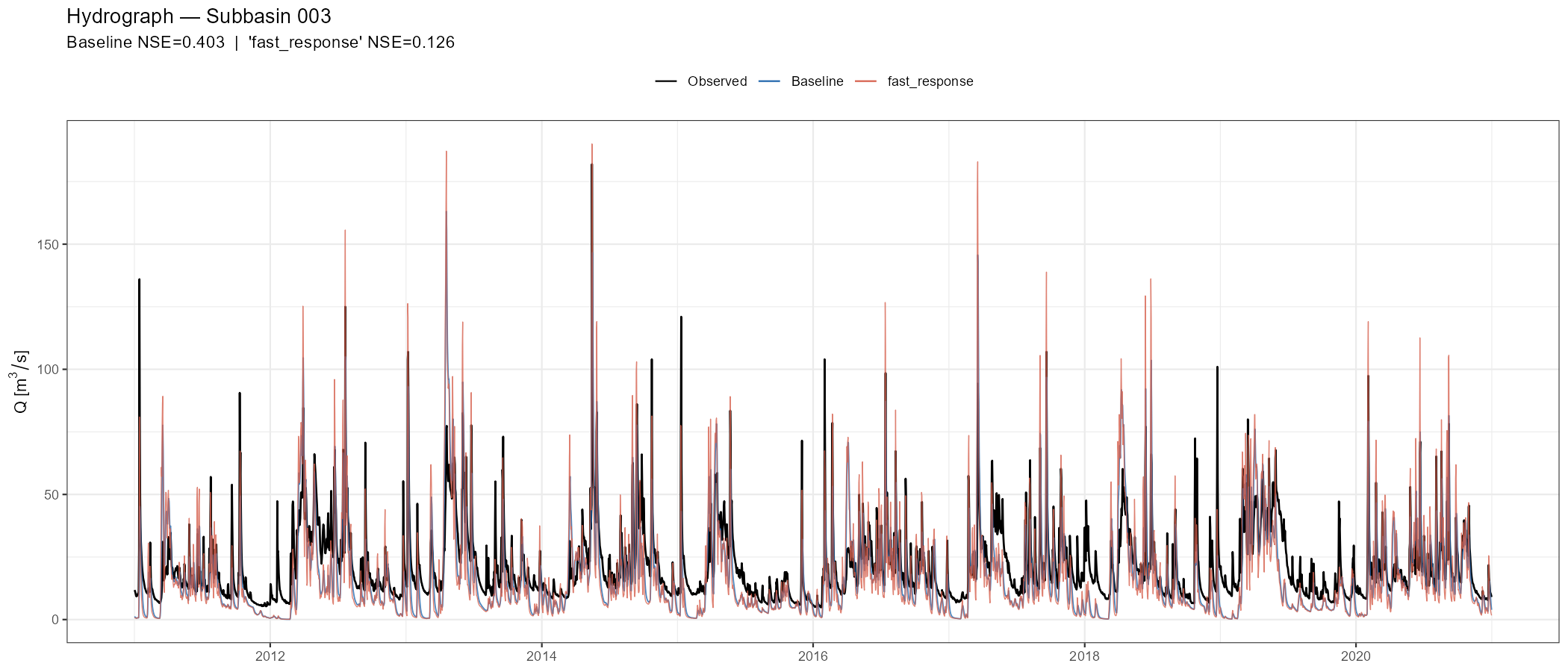
fast_response scenario (orange). Speeding up surface flow slightly sharpens peak response but also introduces false peaks during the recession limb, illustrating how a single parameter change can improve some aspects of the fit while degrading others.
TipUse the Shiny app alongside scripts
After running scenarios in code, load the project in launch_cosero_app() to interactively zoom into specific events, check runoff components, and compare subbasins — without writing additional plot code.
Part 5: Sensitivity Analysis
NoteWhat you’ll learn
Perform a global sensitivity analysis to quantitatively identify which parameters control model output — and which can be fixed at default values. These results directly inform parameter selection for automatic calibration in Module 4.
Why Sensitivity Analysis?
Manual scenario experiments (Part 4) give useful intuition, but they explore parameter space unsystematically. Sensitivity analysis answers the question more rigorously: which parameters most influence model output, and do parameters interact?
This matters practically:
- Focus calibration on the parameters that actually matter
- Fix insensitive parameters at reasonable default values (reduces dimensionality)
- Detect interactions — some parameters only matter in combination
- Understand model behaviour — what processes dominate the response?
Sobol Global Sensitivity Analysis
The CoseRo package implements variance-based Sobol sensitivity analysis, which decomposes the variance of the model output (e.g., NSE) into contributions from individual parameters and their interactions. Unlike one-at-a-time approaches, Sobol analysis varies all parameters simultaneously using quasi-random sampling, capturing the full parameter space.
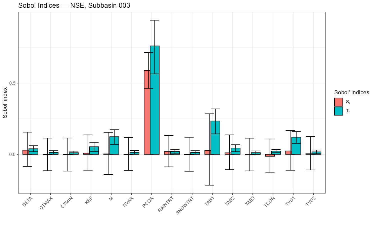
Two indices are computed for each parameter:
- Si (first-order) — the fraction of output variance explained by this parameter alone
- STi (total-effect) — the fraction explained by this parameter including all its interactions with other parameters
The difference STi − Si indicates the strength of parameter interactions.
Available Parameters
The parameter_bounds.csv file defines 31 parameters with their physically plausible ranges, modification types, and categories:
| Category | Parameters | Key role |
|---|---|---|
| Snow | CTMAX, CTMIN, SNOWTRT, RAINTRT, THRT, NVAR, TVAR, GLAC_CT | Snow accumulation and melt and Glacier |
| Soil | M, FK, PWP | Soil water storage |
| Runoff | KBF, BETA, H1, H2, TAB1, TAB2, TVS1, TVS2 | Runoff generation and fast flow |
| Groundwater | TAB3 | Baseflow recession |
| Evapotranspiration | FKFAK, ETSLPCOR, ETSYSCOR, ETVEGCOR | ET partitioning |
| Interception | INTMAX | Canopy storage |
| Precipitation | PCOR, RAINCOR, SNOWCOR | Input correction |
| Temperature | TCOR | Temperature correction |
| Routing | TAB4, TAB5 | Channel routing |
You don’t need to include all 31 in every analysis. Select parameters relevant to your catchment: snow parameters matter more in alpine catchments; soil and ET parameters matter more in lowland basins.
Step 1: Define Parameters and Generate Samples
library(CoseRo)

project_path    <- "C:/COSERO/MyCatchment"
target_subbasin <- "003"

# Select parameters for analysis — adjust to your catchment
# Alpine catchment example: snow + soil + runoff + baseflow + precip correction
param_names <- c("CTMAX", "CTMIN", "RAINTRT", "SNOWTRT", "NVAR", # snow
                 "M", "BETA", "KBF",                             # soil + runoff generation
                 "TAB1", "TAB2", "TAB3", "TVS1", "TVS2",         # flow recession
                 "PCOR", "TCOR")                                 # input correction

# Load bounds and generate Sobol samples
par_bounds   <- load_parameter_bounds(parameters = param_names)
sobol_bounds <- create_sobol_bounds(par_bounds)
samples      <- generate_sobol_samples(sobol_bounds, n = 50, order = "first")
# Total runs = n × (k + 2) = 50 × (15 + 2) = 850
TipChoosing sample size
The base sample size n determines total runs: n × (k + 2) where k is the number of parameters. For 15 parameters, n = 50 gives 850 runs (a few minutes using parallel execution). For robust confidence intervals, use n = 200–500 (several thousand runs). Start small to verify the workflow, then increase.
Step 2: Run Ensemble
base_settings <- list(STARTDATE = "2010 1 1 0 0", ENDDATE = "2020 12 31 0 0",
                      SPINUP = 365, OUTPUTTYPE = 1, PARAFILE = "para_ini.txt")

# Baseline run for reference lines in dotty plots
# statevar_source = 2: warm start — copy statevar.dmp to the input folder first
result_base <- run_cosero(project_path, defaults_settings = base_settings,
                          statevar_source = 2, quiet = TRUE)
baseline_nse <- extract_run_metrics(result_base, target_subbasin, "NSE")
baseline_kge <- extract_run_metrics(result_base, target_subbasin, "KGE")

# Check available cores before choosing n_cores
parallel::detectCores()   # use fewer than total to keep the system responsive

# Parallel ensemble — one project copy per core
ensemble <- run_cosero_ensemble_parallel(
  project_path    = project_path,
  parameter_sets  = samples$parameter_sets,
  par_bounds      = par_bounds,
  base_settings   = base_settings,
  n_cores         = 4,
  statevar_source = 2   # warm start — copy statevar.dmp to input folder first
)

# Persist immediately — runs are expensive and the output can be several GB
saveRDS(ensemble, file.path(project_path, "sensitivity_results", "ensemble.rds"))

# Note: the Wildalpen example figures below used n = 300, k = 15 → 5,100 total runs
TipReloading saved ensemble results
Ensemble runs can take tens of minutes, hours or even days. Save and reload to avoid re-running:
ensemble <- readRDS(file.path(project_path, "sensitivity_results", "ensemble.rds"))Step 3: Compute Indices
# Extract metrics
nse_values <- extract_ensemble_metrics(ensemble, subbasin_id = target_subbasin, metric = "NSE")
kge_values <- extract_ensemble_metrics(ensemble, subbasin_id = target_subbasin, metric = "KGE")

# Calculate Sobol indices with bootstrap confidence intervals
sobol_nse <- calculate_sobol_indices(Y = nse_values, sobol_samples = samples,
                                      boot = TRUE, R = 500)
sobol_kge <- calculate_sobol_indices(Y = kge_values, sobol_samples = samples,
                                      boot = TRUE, R = 500)
Step 4: Visualise Results
The two diagnostic plots are the Sobol index bar chart (which parameters matter?) and the dotty plots (how does performance change across the parameter range?).
# Output directory
plot_dir <- file.path(project_path, "sensitivity_results")
dir.create(plot_dir, showWarnings = FALSE, recursive = TRUE)
sb_tag <- paste0("NB", target_subbasin)
# Sobol index bar plots — the main result
p_sobol_nse <- plot_sobol(sobol_nse,
title = paste("Sobol Indices — NSE, Subbasin", target_subbasin))
print(p_sobol_nse)
ggsave(file.path(plot_dir, paste0("sobol_NSE_", sb_tag, ".png")),
p_sobol_nse, width = 10, height = 6, dpi = 150)
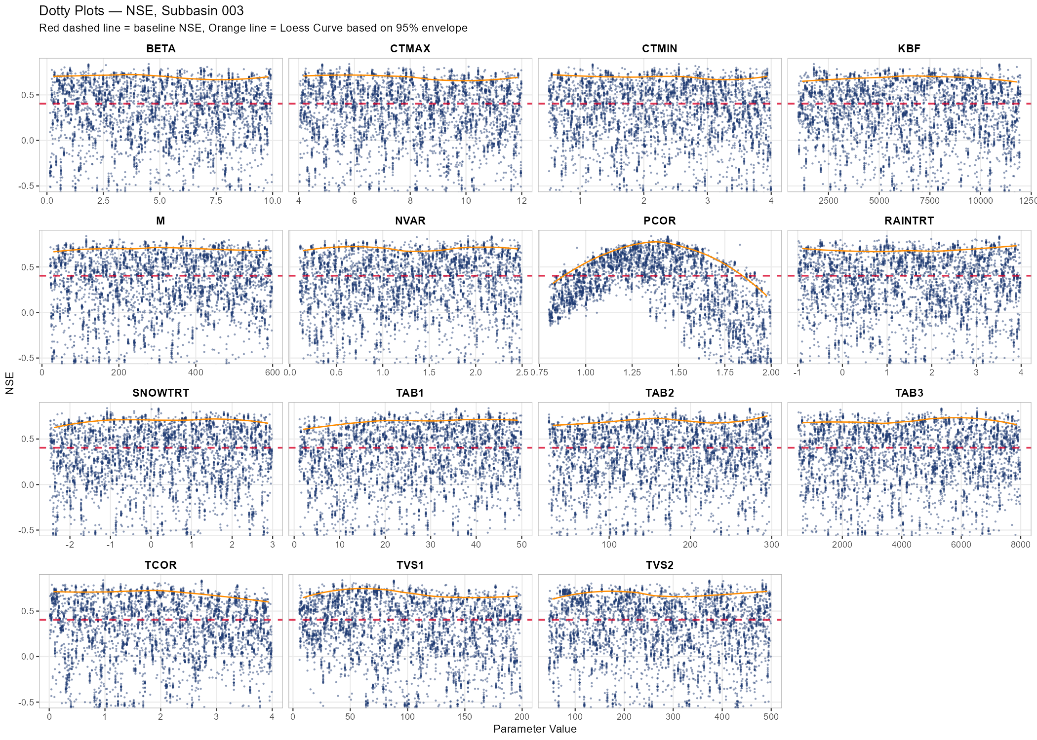
# Dotty plots — parameter identifiability
p_dotty <- plot_dotty(samples$parameter_sets, Y = nse_values, y_label = "NSE",
n_col = 4, reference_line = baseline_nse, y_min = -0.5,
show_envelope = TRUE, envelope_quantile = 0.95) +
labs(title = paste("Dotty Plots — NSE, Subbasin", target_subbasin),
subtitle = "Red dashed line = baseline NSE, Orange line = Loess Curve based on 95% envelope")
print(p_dotty)
ggsave(file.path(plot_dir, paste0("dotty_NSE_", sb_tag, ".png")),
p_dotty, width = 14, height = 10, dpi = 150)What to look for:
- In the Sobol bar chart: parameters with high Si (first-order) have a direct effect. Parameters where STi ≫ Si interact strongly with other parameters. Parameters with low STi (< 0.05) can likely be fixed.
- In the dotty plots: a “valley” or “peak” suggests the parameter is identifiable. A flat cloud means many values work equally well — the parameter is sensitive but not identifiable (equifinality). The orange Loess envelope (95th percentile) highlights the overall response trend across the parameter range.
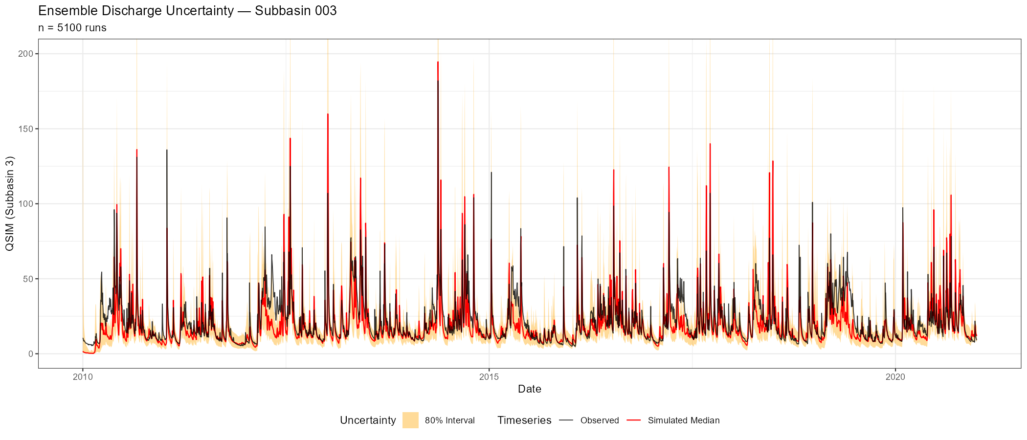
Additional diagnostics (ensemble uncertainty, metric distributions, behavioural ranges) are available for deeper analysis:
Show/hide: Additional sensitivity diagnostics
# Ensemble uncertainty band
p_uncertainty <- plot_ensemble_uncertainty(
ensemble, lower_quantile = 0.1, upper_quantile = 0.9,
date_range = NULL,
q_max = NULL,
subbasin_id = sprintf("%04d", as.numeric(target_subbasin))) +
labs(title = paste("Ensemble Discharge Uncertainty — Subbasin", target_subbasin),
subtitle = sprintf("n = %d runs",
nrow(samples$parameter_sets)))
print(p_uncertainty)
ggsave(file.path(plot_dir, paste0("ensemble_uncertainty_", sb_tag, ".png")),
p_uncertainty, width = 14, height = 6, dpi = 150)
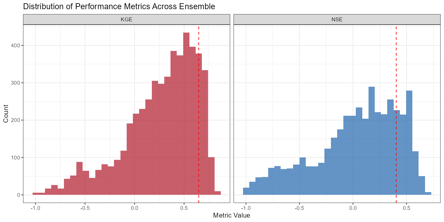
# Metric distributions
metric_df_all <- data.frame(NSE = nse_values, KGE = kge_values) |>
pivot_longer(everything(), names_to = "metric", values_to = "value")
# Filter out extreme outliers (keep everything above -1)
metric_df <- metric_df_all %>%
filter(value >= -1)
p_dist <- ggplot(metric_df, aes(x = value, fill = metric)) +
geom_histogram(bins = 30, alpha = 0.7, position = "identity") +
facet_wrap(~metric, scales = "free_x") +
geom_vline(data = data.frame(metric = c("NSE", "KGE"),
baseline = c(baseline_nse, baseline_kge)),
aes(xintercept = baseline), linetype = "dashed", colour = "red") +
scale_fill_manual(values = c(NSE = "#2166ac", KGE = "#b2182b")) +
labs(title = "Distribution of Performance Metrics Across Ensemble",
x = "Metric Value", y = "Count") +
theme_bw() + theme(legend.position = "none")
print(p_dist)
ggsave(file.path(plot_dir, paste0("metric_distribution_", sb_tag, ".png")),
p_dist, width = 10, height = 5, dpi = 150)
# Behavioural parameter ranges (NSE > threshold)
threshold <- 0.6
behavioural_idx <- which(nse_values > threshold)
all_params <- samples$parameter_sets
behav_params <- samples$parameter_sets[behavioural_idx, , drop = FALSE]
# Stack 'All' and 'Behavioural' sets, pivot to long format, and merge with bounds
df_combined <- bind_rows(
all_params %>% mutate(type = "All"),
behav_params %>% mutate(type = "Behavioural")
) %>%
pivot_longer(cols = all_of(param_names), names_to = "parameter", values_to = "value") %>%
left_join(par_bounds %>% select(parameter, min, max, modification_type), by = "parameter")
# Apply normalization and calculate all quantiles in one clean block
summary_stats <- df_combined %>%
mutate(
# Log scale if min > 0 and max spans > 1 order of magnitude
is_log = (min > 0 & (max / min) > 10),
norm_value = if_else(is_log,
(log10(pmax(value, min)) - log10(min)) / (log10(max) - log10(min)),
(value - min) / (max - min))
) %>%
group_by(parameter, type, modification_type) %>%
summarise(
q00 = min(value, na.rm = TRUE),
q25 = quantile(value, 0.25, na.rm = TRUE),
q50 = quantile(value, 0.50, na.rm = TRUE),
q75 = quantile(value, 0.75, na.rm = TRUE),
q100 = max(value, na.rm = TRUE),
norm_q25 = quantile(norm_value, 0.25, na.rm = TRUE),
norm_q50 = quantile(norm_value, 0.50, na.rm = TRUE),
norm_q75 = quantile(norm_value, 0.75, na.rm = TRUE),
.groups = "drop"
)
# Calculate current (a priori) values and normalize them
cur_vals <- read_parameter_table(par_file, param_names, zone_id = "all")
cur_summary <- cur_vals %>%
pivot_longer(cols = all_of(param_names), names_to = "parameter", values_to = "value") %>%
left_join(par_bounds %>% select(parameter, min, max), by = "parameter") %>%
mutate(
is_log = (min > 0 & (max / min) > 10),
norm_value = if_else(is_log,
(log10(pmax(value, min)) - log10(min)) / (log10(max) - log10(min)),
(value - min) / (max - min))
) %>%
group_by(parameter) %>%
summarise(
cur_mean = mean(value, na.rm = TRUE),
cur_norm_q25 = quantile(norm_value, 0.25, na.rm = TRUE),
cur_norm_q50 = quantile(norm_value, 0.50, na.rm = TRUE),
cur_norm_q75 = quantile(norm_value, 0.75, na.rm = TRUE),
.groups = "drop"
)
# Normalised ranges plot
p_ranges <- ggplot(summary_stats, aes(x = parameter, y = norm_q50, colour = type)) +
geom_pointrange(aes(ymin = norm_q25, ymax = norm_q75),
position = position_dodge(width = 0.5), linewidth = 0.8) +
geom_pointrange(data = cur_summary,
aes(x = parameter, y = cur_norm_q50, ymin = cur_norm_q25, ymax = cur_norm_q75),
inherit.aes = FALSE, shape = 18, size = 0.5, linewidth = 0.8, colour = "#2166ac") +
geom_hline(yintercept = c(0, 1), linetype = "dotted", colour = "grey60") +
scale_colour_manual(values = c(All = "grey50", Behavioural = "#e74c3c")) +
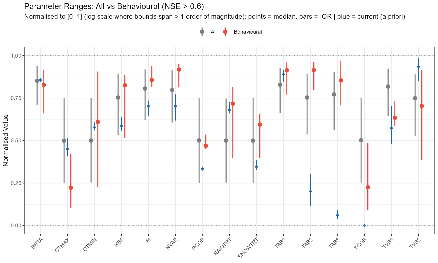
labs(title = sprintf("Parameter Ranges: All vs Behavioural (NSE > %.1f)", threshold),
subtitle = "Normalised to [0, 1] (log scale where bounds span > 1 order of magnitude); points = median, bars = IQR | blue = current (a priori)",
x = NULL, y = "Normalised Value", colour = NULL) +
theme_bw() +
theme(axis.text.x = element_text(angle = 45, hjust = 1), legend.position = "top")
print(p_ranges)
ggsave(file.path(plot_dir, paste0("behavioural_ranges_", sb_tag, ".png")),
p_ranges, width = 10, height = 6, dpi = 150)
# Absolute values plot: one panel per parameter, free y-scale
p_abs <- ggplot(summary_stats, aes(x = type, y = q50, colour = type)) +
# Thin line showing the absolute Min to Max
geom_linerange(aes(ymin = q00, ymax = q100), linewidth = 0.3, alpha = 0.6) +
# Thick line showing the IQR (middle 50%)
geom_pointrange(aes(ymin = q25, ymax = q75), linewidth = 1.0) +
# Add the a priori mean
geom_hline(data = cur_summary, aes(yintercept = cur_mean),
colour = "#2166ac", linetype = "dashed", linewidth = 0.7) +
facet_wrap(~parameter, scales = "free_y", ncol = 5) +
scale_colour_manual(values = c(All = "grey50", Behavioural = "#e74c3c")) +
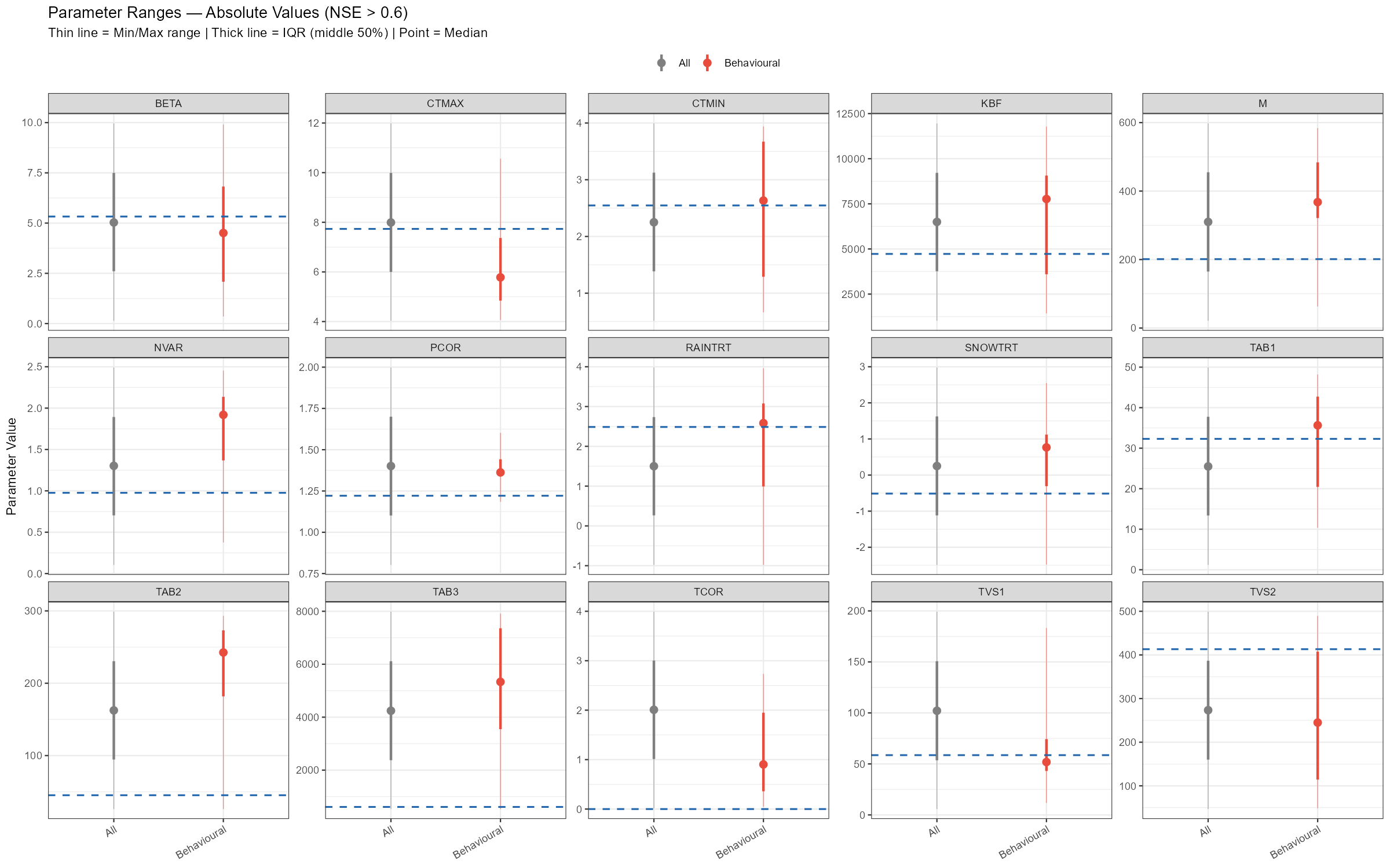
labs(title = sprintf("Parameter Ranges — Absolute Values (NSE > %.1f)", threshold),
subtitle = "Thin line = Min/Max range | Thick line = IQR (middle 50%) | Point = Median | Blue dashed = current mean",
x = NULL, y = "Parameter Value", colour = NULL) +
theme_bw() +
theme(legend.position = "top", axis.text.x = element_text(angle = 30, hjust = 1))
print(p_abs)
ggsave(file.path(plot_dir, paste0("behavioural_absolute_", sb_tag, ".png")),
p_abs, width = 16, height = 10, dpi = 150)
# Adjustment summary table
# relchg params: adjustment = behav_median / current_mean (multiplicative factor)
# abschg params: adjustment = behav_median - current_mean (additive offset)
adj_summary <- summary_stats %>%
filter(type == "Behavioural") %>%
select(parameter, mod_type = modification_type,
behav_q25 = q25, behav_median = q50, behav_q75 = q75) %>%
left_join(cur_summary %>% select(parameter, current_mean = cur_mean), by = "parameter") %>%
mutate(
adjustment = if_else(mod_type == "relchg",
behav_median / current_mean,
behav_median - current_mean),
adj_type = if_else(mod_type == "relchg", "x (factor)", "delta (offset)"),
across(where(is.numeric), ~round(., 3))
) %>%
select(parameter, mod_type, current_mean, behav_q25, behav_median, behav_q75,
adjustment, adj_type)
cat(sprintf("\n--- Adjustment Summary: current → behavioural median (NSE > %.1f) ---\n",
threshold))
print(adj_summary, row.names = FALSE)
write.csv(adj_summary,
file.path(plot_dir, paste0("adjustment_summary_", sb_tag, ".csv")),
row.names = FALSE)Interpreting Sobol Results
Results are metric-dependent: a parameter that is sensitive for NSE may be insensitive for KGE (which also weights bias and variability). Running the analysis for both metrics is therefore recommended.
Example: Wildalpen Catchment
The following figures show the sensitivity workflow applied to the Wildalpen example catchment (subbasin 003, outlet), using n = 300 Sobol samples and 15 parameters (5,100 total model runs).
The adjustment summary table below quantifies the implied calibration direction for each parameter, based on the median and for subbasin 3. For relchg parameters the adjustment is a multiplicative factor; for abschg parameters it is an additive offset applied to the spatial mean.
| Parameter | Current mean | Behavioural median | Adjustment | Type |
|---|---|---|---|---|
| BETA | 5.33 | 4.51 | ×0.85 | relchg |
| CTMAX | 7.73 | 5.78 | ×0.75 | relchg |
| CTMIN | 2.55 | 2.63 | ×1.03 | relchg |
| KBF | 4 725 | 7 768 | ×1.64 | relchg |
| M | 201 | 368 | ×1.83 | relchg |
| NVAR | 0.98 | 1.92 | ×1.97 | relchg |
| PCOR | 1.22 | 1.36 | ×1.12 | relchg |
| RAINTRT | 2.49 | 2.58 | +0.10 | abschg |
| SNOWTRT | −0.51 | 0.77 | +1.28 | abschg |
| TAB1 | 32.3 | 35.6 | ×1.10 | relchg |
| TAB2 | 45.2 | 243 | ×5.37 | relchg |
| TAB3 | 610 | 5 334 | ×8.75 | relchg |
| TCOR | 0 | 0.90 | +0.90 | abschg |
| TVS1 | 58.6 | 51.8 | ×0.89 | relchg |
| TVS2 | 413 | 245 | ×0.59 | relchg |
TAB3 (×8.75) and TAB2 (×5.37) stand out as the largest adjustments — the a priori baseflow and subsurface recession constants seem to be too fast for this catchment. M (×1.83) and NVAR (×1.97) also need substantial increases, while CTMAX (×0.75) and TVS2 (×0.59) should be reduced. SNOWTRT and TCOR require positive temperature offsets, consistent with a cold alpine environment. PCOR (×1.12) confirms a modest but systematic precipitation underestimation.
Exporting Results
export_sensitivity_results(
  output_dir     = file.path(project_path, "sensitivity_results"),
  sobol_indices  = sobol_nse,
  parameter_sets = samples$parameter_sets,
  metrics        = nse_values,
  prefix         = paste0("sobol_NSE_NB", target_subbasin)
)
NoteSensitivity ≠ Identifiability
A parameter can be sensitive (it strongly affects the output) yet poorly identifiable (many different values produce similar performance). The dotty plots help detect this: a clear “optimum” in the scatter suggests identifiability; a flat cloud does not. Equifinality — multiple parameter combinations yielding similar performance — is the norm rather than the exception in hydrological modelling.
TipFrom sensitivity to calibration
In Module 4, you will use the Sobol results to select which parameters to calibrate and optionally narrow their bounds. Parameters with high sensitivity indices are candidates for calibration; insensitive parameters can be fixed at their default values to reduce the search space. Nevertheless, results from the ensemble runs can be used to choose good working models.
Part 6: Behavioural Run Filtering
The Sobol analysis answers which parameters matter and how much. A complementary question is: which runs actually produce acceptable simulations?
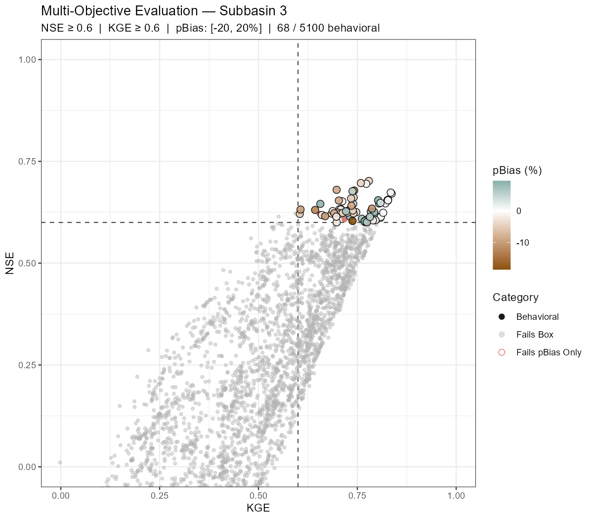
Behavioural filtering applies simultaneous thresholds on multiple performance metrics — here NSE, KGE, and percent bias — to classify every ensemble run into one of three categories:
- Behavioral — passes all three criteria
- Fails pBias Only — passes the NSE/KGE box but has a systematic bias outside the acceptable range
- Outside Box — fails NSE and/or KGE threshold
The extract_behavioral_runs() function does this in one call. It returns a filtered ensemble object that can be passed directly to plot_dotty() or calculate_sobol_indices() to restrict downstream analysis to acceptable runs only.
NoteSelection vs. plotting arguments
The three threshold arguments (nse_thresh, kge_thresh, pbias_thresh) are the only ones that control which runs are classified as behavioural. The remaining arguments (plot_uncertainty, date_range, q_max, lower_quantile, upper_quantile) are passed via ... to plot_ensemble_uncertainty and affect only the hydrograph plot — they have no effect on the selection.
# Selection criteria — these three thresholds determine which runs are "behavioural":
# nse_thresh / kge_thresh / pbias_thresh → used for filtering only
#
# Plotting-only arguments (passed via ... to plot_ensemble_uncertainty, no effect on selection):
# plot_uncertainty → if TRUE, also render the uncertainty hydrograph for behavioural runs
# date_range → x-axis window of the hydrograph; does NOT filter the metric computation
# q_max → y-axis cap on the hydrograph
# lower_quantile / upper_quantile → uncertainty band width on the hydrograph
eval_out <- extract_behavioral_runs(
ensemble_output = ensemble,
subbasin_id = target_subbasin,
nse_thresh = 0.6, # behavioural threshold
kge_thresh = 0.6, # behavioural threshold
pbias_thresh = c(-20, 20), # behavioural threshold
plot_uncertainty = TRUE,
date_range = c("2015-01-01", "2020-12-31"), # hydrograph x-axis only
q_max = 200, # hydrograph y-axis cap
lower_quantile = 0, # uncertainty band (plot only)
upper_quantile = 1, # uncertainty band (plot only)
xlim = c(0, 1), # KGE x-axis
ylim = c(0, 1) # NSE y-axis
)
# How many runs passed all criteria?
n_behav <- length(eval_out$behavioral_run_ids)
n_total <- length(ensemble$results)
cat(sprintf("Behavioural runs: %d / %d (%.1f%%)\n", n_behav, n_total,
100 * n_behav / n_total))
# Scatter plot and uncertainty hydrograph
print(eval_out$scatter_plot)
print(eval_out$uncertainty_plot)
# Save
ggsave(file.path(plot_dir, paste0("behavioral_scatter_", sb_tag, ".png")),
eval_out$scatter_plot, width = 8, height = 7, dpi = 150)
ggsave(file.path(plot_dir, paste0("behavioral_uncertainty_", sb_tag, ".png")),
eval_out$uncertainty_plot, width = 14, height = 6, dpi = 150)
# Dotty plots restricted to behavioural runs only
behav_nse <- eval_out$metrics_df$NSE[eval_out$metrics_df$category == "Behavioral"]
p_dotty_behav <- plot_dotty(
eval_out$filtered_ensemble$parameter_sets,
Y = behav_nse,
y_label = "NSE",
n_col = 4,
reference_line = 0.6,
y_min = 0.5,
show_envelope = TRUE,
envelope_quantile = 1
) +
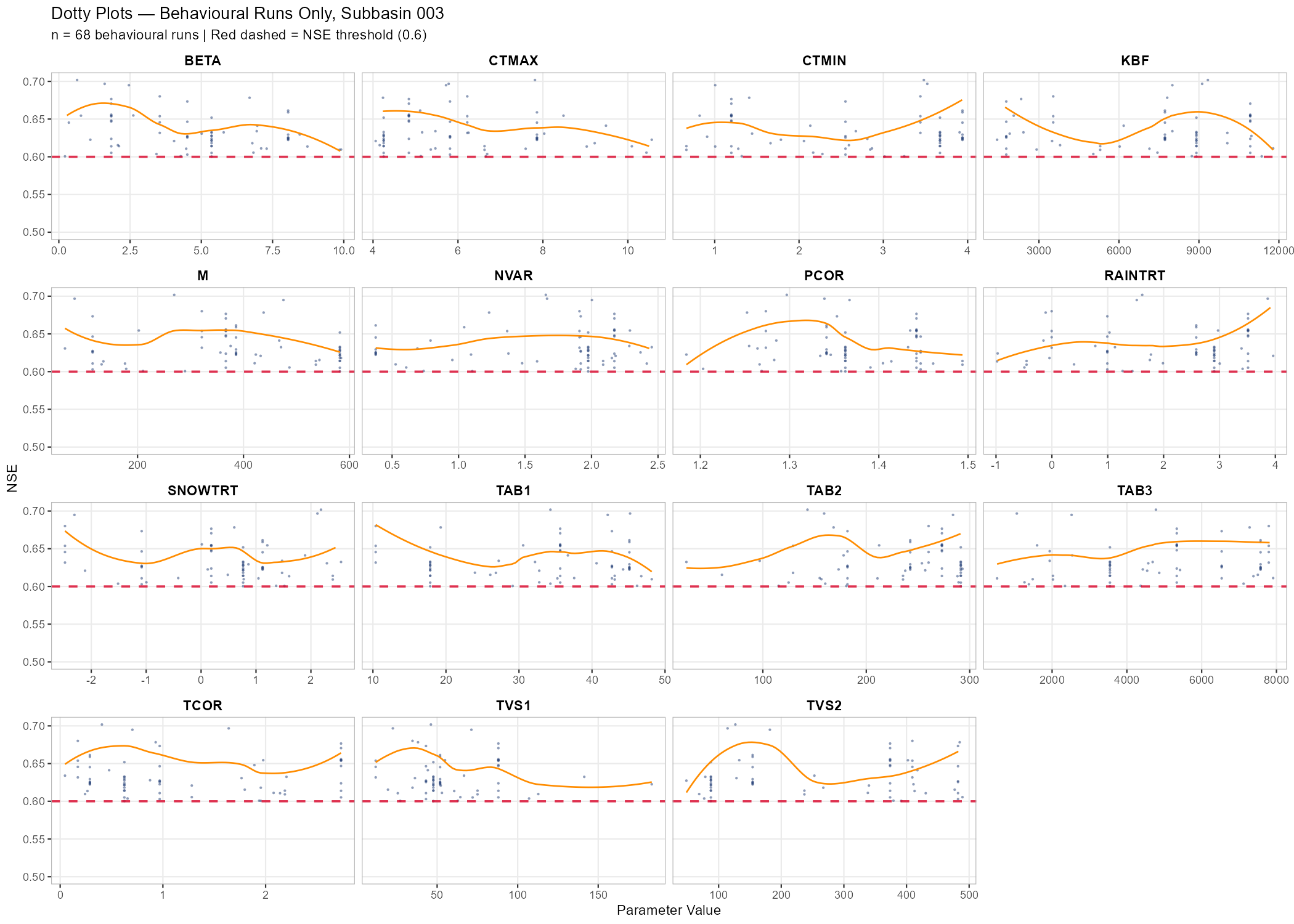
labs(title = paste("Dotty Plots — Behavioural Runs Only, Subbasin", target_subbasin),
subtitle = sprintf("n = %d behavioural runs | Red dashed = NSE threshold (0.6)", n_behav))
print(p_dotty_behav)
ggsave(file.path(plot_dir, paste0("dotty_behavioural_", sb_tag, ".png")),
p_dotty_behav, width = 14, height = 10, dpi = 150)Example: Wildalpen Catchment
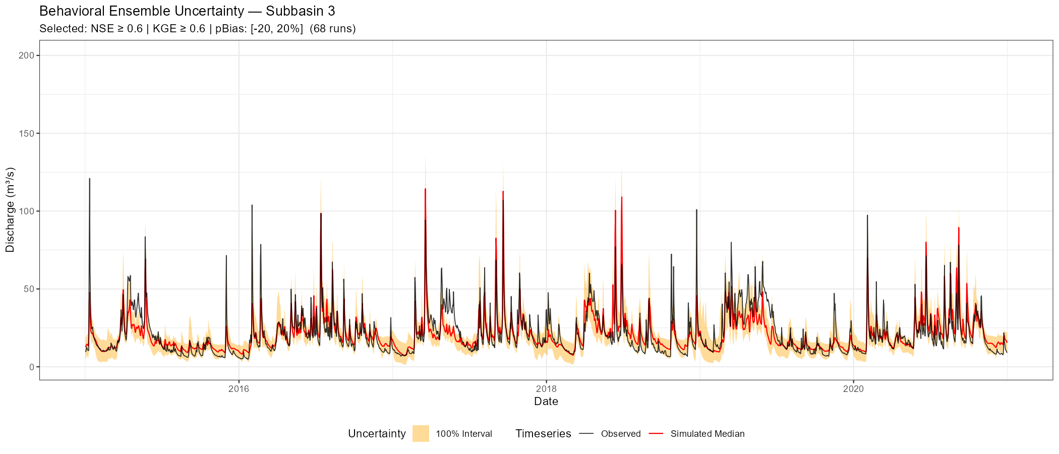
The following figures show behavioural filtering applied to the Wildalpen example (subbasin 003, thresholds: NSE ≥ 0.6, KGE ≥ 0.6, pBias ∈ [−20%, +20%]).
Saving the Best-Performing Parameter Set
After identifying which runs are behavioural, it is useful to extract and save the single best-performing parameter set — for example, the run with the highest NSE or KGE — as a COSERO parameter file. This file can then serve as a warm-start point for Module 4 calibration or as a quick reference for the best hand-tuned solution found during sensitivity analysis.
The run_id in eval_out$metrics_df is a 1-based positional index into the original ensemble (and therefore into samples$parameter_sets). The saved file is produced with modify_parameter_table(), which applies a Spatial Mean Strategy to distribute the scalar ensemble values across zones:
relchg:factor = sampled_value / spatial_mean; each zone value is multiplied by that factor.abschg:offset = sampled_value - spatial_mean; the offset is added uniformly to all zones.
In both cases the spatial heterogeneity encoded in the base parameter file is preserved while the catchment-average equals the sampled value. This is identical to what the ensemble runner applied during simulation, guaranteeing full consistency between the written file and the run result.
# --- Identify best run by NSE ---
best_idx_nse <- which.max(eval_out$metrics_df$NSE)
best_run_id  <- eval_out$metrics_df$run_id[best_idx_nse]
best_nse     <- eval_out$metrics_df$NSE[best_idx_nse]
best_kge     <- eval_out$metrics_df$KGE[best_idx_nse]
cat(sprintf("Best NSE run: id = %d  |  NSE = %.4f  |  KGE = %.4f\n",
            best_run_id, best_nse, best_kge))

# --- Identify best run by KGE ---
best_idx_kge    <- which.max(eval_out$metrics_df$KGE)
best_run_id_kge <- eval_out$metrics_df$run_id[best_idx_kge]
best_kge_val    <- eval_out$metrics_df$KGE[best_idx_kge]
cat(sprintf("Best KGE run: id = %d  |  KGE = %.4f  |  NSE = %.4f\n",
            best_run_id_kge, best_kge_val, eval_out$metrics_df$NSE[best_idx_kge]))

# --- Write best NSE parameter file ---
# Scalar values = catchment-average targets. modify_parameter_table() distributes them:
#   relchg → factor = sampled / spatial_mean;  zone_i = zone_i_orig * factor
#   abschg → offset = sampled - spatial_mean;  zone_i = zone_i_orig + offset
# Spatial heterogeneity of the base file is preserved; same logic as the ensemble runner.
best_params_nse   <- as.list(samples$parameter_sets[best_run_id, , drop = FALSE][1, ])
par_file_best_nse <- file.path(project_path, "input", "para_best_NSE.txt")
file.copy(par_file, par_file_best_nse, overwrite = TRUE)
orig_vals_best <- read_parameter_table(par_file_best_nse, par_bounds$parameter, zone_id = "all")
modify_parameter_table(par_file_best_nse, best_params_nse, par_bounds, orig_vals_best,
                       add_timestamp = TRUE)
cat("Saved best NSE parameter file to:", par_file_best_nse, "\n")

# --- Write best KGE parameter file (only if different from best NSE run) ---
if (best_run_id_kge != best_run_id) {
  best_params_kge   <- as.list(samples$parameter_sets[best_run_id_kge, , drop = FALSE][1, ])
  par_file_best_kge <- file.path(project_path, "input", "para_best_KGE.txt")
  file.copy(par_file, par_file_best_kge, overwrite = TRUE)
  orig_vals_kge <- read_parameter_table(par_file_best_kge, par_bounds$parameter, zone_id = "all")
  modify_parameter_table(par_file_best_kge, best_params_kge, par_bounds, orig_vals_kge,
                         add_timestamp = TRUE)
  cat("Saved best KGE parameter file to:", par_file_best_kge, "\n")
} else {
  cat("Best NSE and best KGE are the same run — no separate KGE file written.\n")
}

# --- Optional verification: re-run COSERO with the saved parameter file ---
# Uncomment to confirm the saved file reproduces the ensemble run result.
# result_best <- run_cosero(
#   project_path      = project_path,
#   defaults_settings = modifyList(base_settings, list(PARAFILE = "para_best_NSE.txt")),
#   statevar_source   = 2
# )
# cat(sprintf("Verification — NSE = %.4f  |  KGE = %.4f\n",
#             extract_run_metrics(result_best, target_subbasin, "NSE"),
#             extract_run_metrics(result_best, target_subbasin, "KGE")))
What You Should Know
After completing this module you should understand the following concepts and be able to reproduce the corresponding steps for your own catchment. These points may also serve as a guide for your presentation.
- Initial run diagnostics: Interpret a hydrograph and performance metrics (NSE, KGE, volume bias) from an a priori parameter run. Explain what “good” and “poor” performance means and why the uncalibrated model may not reproduce observed discharge well.
- Shiny app exploration: Navigate the CoseRo app to inspect hydrographs, runoff components, and performance across subbasins. Modify a parameter interactively and explain how the simulated discharge responds.
- Scenario comparison: Set up and run at least three parameter scenarios. Explain why results differ across scenarios and which parameter changes had the largest effect on performance — and why.
- Sensitivity analysis: Read and interpret Sobol index bar charts and dotty plots. Distinguish between sensitive and insensitive parameters, and between identifiable and non-identifiable parameters. Explain the concept of equifinality in your own words.
- Behavioural filtering: Explain the principle of multi-objective behavioural filtering. Describe what the KGE vs. NSE scatter plot shows and how the three threshold criteria interact. Discuss how the dotty plot changes when restricted to behavioural runs.
- Best parameter set: Explain why the best single run from an ensemble is not the same as a calibrated parameter set, and what it can and cannot be used for. Verify that
para_best_NSE.txtwas written and reproduces the expected metrics. - Synthesis: Reflect on which parameters you would select for calibration in Module 4, based on the sensitivity and behavioural filtering results, and justify your choice.
Document created: 2026-05-22
References
Gupta, H. V., Kling, H., Yilmaz, K. K., and Martinez, G. F.: Decomposition of the mean squared error and NSE performance criteria: Implications for improving hydrological modeling, Journal of Hydrology, 377, 80–91, 2009.
Kirchner, J. W.: Getting the right answers for the right reasons: Linking measurements, analyses, and models to advance the science of hydrology, Water Resources Research, 42, W03S04, https://doi.org/10.1029/2005WR004362, 2006.
Klemeš, V.: Dilettantism in hydrology: Transition or destiny?, Water Resources Research, 22, S177–S188, https://doi.org/10.1029/WR022i09Sp0177S, 1986.
Knoben, W. J. M., Freer, J. E., and Woods, R. A.: Technical note: Inherent benchmark or not? Comparing Nash–Sutcliffe and Kling–Gupta efficiency scores, Hydrology and Earth System Sciences, 23, 4323–4331, https://doi.org/10.5194/hess-23-4323-2019, 2019.
Nash, J. E. and Sutcliffe, J. V.: River flow forecasting through conceptual models. Part I: A discussion of principles, Journal of Hydrology, 10, 282–290, 1970.