Show code
install.packages("remotes")
remotes::install_github("Herrnegger/CoseRo")Mathew Herrnegger · mathew.herrnegger@boku.ac.at
Institute of Hydrology and Water Management (HyWa) BOKU University Vienna, Austria
LAWI301236 · Distributed Hydrological Modeling with COSERO
![]()
Hydrological models serve as a objective link between our theoretical understanding of the water cycle and real-world applications. They provide the necessary basis for objective decision-making in water resources management and are important tools for scientific research.
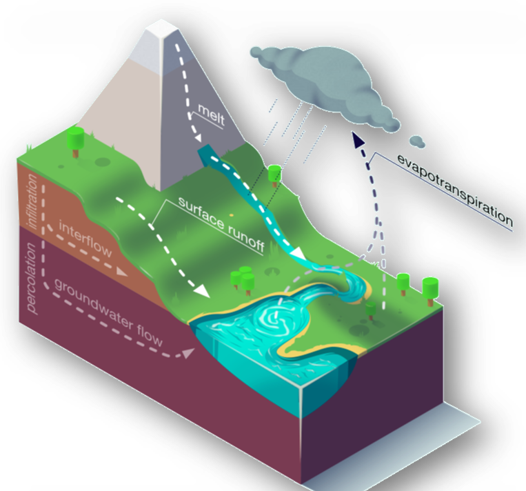
By translating complex fluxes—such as precipitation, snowmelt, evapotranspiration, and subsurface flows—into quantifiable river discharge, models allow us to answer questions regarding safety, availability, and sustainability of water.
Domains of application include:
The fundamental problem of rainfall-runoff modelling can be described as a non-linear transformation of driving meteorological inputs into catchment runoff. The model must effectively translate inputs like Precipitation, Temperature, and Potential Evapotranspiration into a discharge output.
This transformation is complex because the relationship between rainfall and runoff is not constant; it is a dynamic function \(f\) influenced by different factors:
To make things even more complicated, these relationships and dependencies are not constant and change over time.
To address the complexities of the hydrological cycle, hydrological models like COSERO explicitly represents storage components, process interactions, and anthropogenic diversions. This module introduces distributed hydrological modeling using the CoseRo R interface, with a focus on Austrian catchments.
Learning Objectives:
![]() The COSERO model (COntinuous SEmi-distributed RunOff) is a continuous, (semi-)distributed, conceptual rainfall-runoff model developed at the Institute of Hydrology and Water Management (HyWa), formerly IWHW, at BOKU University Vienna, Austria. The model concept is similar to the HBV model (Bergström, 1992) and accounts for accumulation and melting of snow and glaciers, actual evapotranspiration, interception, soil water storage, separation of runoff into different flow components, and routing by means of a cascade of linear and non-linear reservoirs.
The COSERO model (COntinuous SEmi-distributed RunOff) is a continuous, (semi-)distributed, conceptual rainfall-runoff model developed at the Institute of Hydrology and Water Management (HyWa), formerly IWHW, at BOKU University Vienna, Austria. The model concept is similar to the HBV model (Bergström, 1992) and accounts for accumulation and melting of snow and glaciers, actual evapotranspiration, interception, soil water storage, separation of runoff into different flow components, and routing by means of a cascade of linear and non-linear reservoirs.
Over the years, many people have worked on COSERO, which evolved from a model structure originally developed for forecasting runoff of the river Enns in Austria (Nachtnebel et al., 1993). Subsequently, the model has undergone substantial improvements including enhanced snow modules, automatic parameter calibration, and modifications for real-time flood forecasting, distributed routing, or trans-catchment diversions.
Current development at BOKU-HyWa focuses on regionalization strategies and parameter optimization using spatially distributed catchment data—such as elevation, slope, aspect, land use, or soil—to estimate model parameters via a priori defined transfer functions (Feigl et al., 2020, 2022, 2026; Klotz et al., 2017b). This approach, similar to the Multiscale Parameter Regionalization (MPR) proposed by Samaniego et al. (2010), significantly reduces the number of parameters required for optimization and helps overcome scale dependency, while a second development avenue utilizes Machine-Learning based parameter fields (Zeitfogel et al., 2023; Zeitfogel et al., 2025).
Parallel to these scientific advancements, the model code has been technically modernized through OpenMP-based parallelization and dynamical array allocation to support high-resolution simulations of large regions, alongside architectural enhancements such as modularized subroutines, global variable definitions, and improved process representations for glacier melt and anthropogenic diversions.
The COSERO Handbook is the primary reference document for the model. It describes the model structure, all process equations, input/output file formats, and configuration options in detail. Refer to it whenever you need the mathematical formulation behind a process or want to understand what a specific parameter controls.
Since 1993, different versions of COSERO have been successfully applied in numerous scientific and commercial projects all over the world, including:
| Category | Selected References |
|---|---|
| Climate Change Impact Assessment | APCC (2014); Buttinger (2018); Ehrendorfer et al. (2024); Friedrichs-Manthey et al. (2024); Herrnegger et al. (2018b); Kiesel et al. (2020); Kling et al. (2012); Mehdi et al. (2021); Nachtnebel et al. (2011); Stanzel and Nachtnebel (2010); Stanzel et al. (2018); Stanzel and Kling (2018); Buttinger et al. (2018) |
| Flood Forecasting & Real-Time Applications | Martin Santos et al. (2019); Martin Santos et al. (2020); Martin Santos et al. (2021); Nachtnebel and Kahl (2008); Nachtnebel et al. (2009a); Nachtnebel et al. (2009b); Nachtnebel et al. (2010); Nachtnebel et al. (2013); Pulka et al. (2021); Pulka (2021); Pulka et al. (2022); Stanzel et al. (2008); Wesemann et al. (2018b); Wesemann (2021) |
| Water Balance Studies | Herrnegger and Nachtnebel (2011); Herrnegger and Nachtnebel (2012a); Herrnegger et al. (2020); Kling (2006); Zeitfogel et al. (2024b); Zeitfogel et al. (2025) |
| Large-Sample Hydrology & Data | Kling et al. (2015); Klingler (2020); Klingler et al. (2021); Konold et al. (2025) |
| Precipitation Analysis & Correction | Bica et al. (2011); Herrnegger and Nachtnebel (2012b); Herrnegger and Nachtnebel (2012c); Herrnegger (2013); Herrnegger et al. (2015); Herrnegger et al. (2018a); Maier et al. (2024); Maier et al. (2026); Omonge et al. (2022); Omonge et al. (2019); Pulka et al. (2023); Pulka et al. (2024) |
| Hydrological Modeling & Applications | BMFLUW (2005); Eder et al. (2005); Enzinger (2009); Feiel (2018); Fuchs (1998); Guse et al. (2019); Herrnegger et al. (2020); Kling et al. (2006); Kling et al. (2014); Lerche (2022); Nachtnebel et al. (1993); Schößwendter (2018); Stanzel (2012); Wesemann et al. (2018b); Wesemann (2021) |
| Model Development & Parameterization | Burgholzer (2017); Ehrendorfer (2022); Ehrendorfer and Herrnegger (2022); Ehrendorfer and Herrnegger (2023); Ehrendorfer et al. (2023); Frey and Holzmann (2015); Fuchs (1998); Haberl (2021); Kling (2002); Kling and Nachtnebel (2009); Klotz et al. (2015); Klotz et al. (2017a); Klotz et al. (2017b); Salamon (2020); Schulz et al. (2015); Stanzel (2012); Wesemann et al. (2018a); Zeitfogel et al. (2022); Zeitfogel et al. (2024a); Zeitfogel et al. (2024b); Zeitfogel et al. (2025) |
COSERO is a flexible model able to simulate different hydrological systems across a wide range of scales and resolutions. Its spatial scalability—from lumped to semi-distributed and distributed setups—allows for applications ranging from small plot scales to large catchments covering thousands of square kilometers, while its temporal flexibility supports resolutions from 15-minute intervals for real-time flood forecasting to monthly time steps for long-term water balance studies. The model provides a comprehensive process representation, accounting for the accumulation and melting of snow and glaciers, actual evapotranspiration, interception, soil water storage, and routing via linear and non-linear reservoirs. Additionally, the model was also applied in an inverse modeling approach, utilizing runoff observations as input to calculate areal rainfall (Herrnegger, 2013; Herrnegger et al., 2015).
COSERO accounts for accumulation and melting of snow and glaciers, actual evapotranspiration from interception, snow and soil layer, storage of water in the soil, and separation of runoff into different runoff components (surface flow, interflow and baseflow) by means of a cascade of linear and non-linear reservoirs. The model is spatially distributed - all inputs, outputs and parameters have a spatial dimension.
COSERO is formulated in a state-space formulation with state transition functions:
\[ \dot{S}_t = f(\dot{S}_{t-1}, \dot{I}_t) \tag{1}\]
and output functions:
\[ \dot{O}_t = g(\dot{S}_{t-1}, \dot{I}_t) \tag{2}\]
where:
| Symbol | Units | Description |
|---|---|---|
| \(\dot{I}_t\) | mm/Δt | Input |
| \(\dot{O}_t\) | mm/Δt | Output |
| \(\dot{S}_t\) | mm | System states |
| Δt | - | Model time step |
The state transition function (Equation 1) describes how the state variables change from one time step to the next, based on the previous state and the current inputs. The output function (Equation 2) relates the state variables to the hydrological outputs of interest, such as streamflow, groundwater levels, or reservoir storage. State-space formulations are commonly used in hydrological modeling to represent the dynamic behavior of the hydrological cycle and the state variables typically represent different components of the water cycle, such as soil moisture, groundwater storage, snow accumulation, and surface water storage.
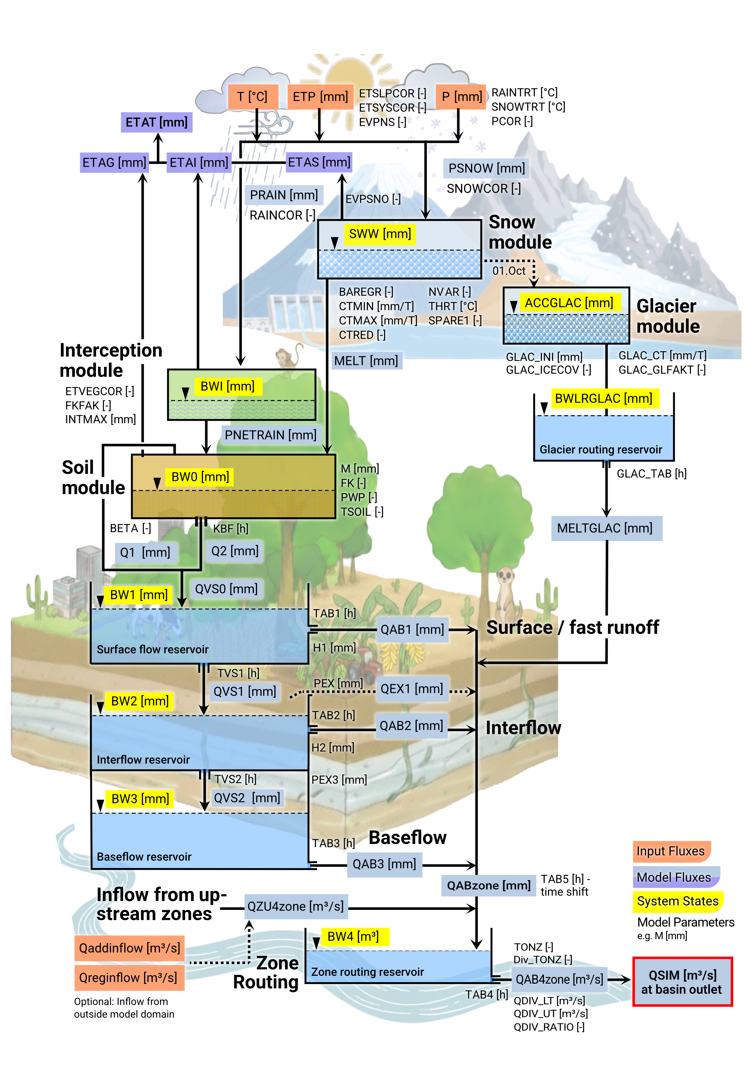
The COSERO model (Figure 2) integrates continuous hydrological processes through five interconnected modules: Snow, Glacier, Interception, Soil, and Routing. The schematic distinguishes between Input Fluxes (orange, e.g., \(P, T\)), System States (yellow, e.g., \(BW0\) soil moisture, \(SWW\) snow water equivalent), and Model Fluxes (blue/black arrows).
SNOWTRT and RAINTRT. To account for sub-grid variability in alpine terrain, snowfall is distributed log-normally across internal elevation classes (controlled by NVAR).CTMIN (Dec 21) and CTMAX (Jun 21) to simulate albedo decay.GLAC_CT and considering long-term hourly radiation and initiates only after seasonal snow depletion.INTMAX) captures precipitation; excess water reaches the soil as throughfall.ETSLPCOR), vegetation (ETVEGCOR), and soil moisture (FKFAK).M, FK, PWP and state \(BW0\)) generates surface runoff (\(Q1\)) via a non-linear function of soil moisture (controlled by parameter BETA) and percolation (\(Q2\)) to subsurface storage (controlled by KBF) ).Total discharge (\(Q_{sim}\)) is the sum of three parallel flow components plus glacier melt:
TAB1). Outflow occurs only when storage exceeds the threshold H1, while vertical percolation to the interflow zone is controlled by TVS1.TAB2). Outflow occurs when storage exceeds the threshold H2, with further percolation to the baseflow zone governed by TVS2.TAB3), representing the long-term baseflow component.These components are routed through a cascade of linear reservoirs (Zone Routing). The model also supports anthropogenic diversions with parameters Div_TONZ, QDIV_LT and QDIV_UT, allowing runoff redistribution for complex canal or hydropower systems (Wesemann et al., 2018b).
The following tables provide an overview of the system states, fluxes, and governing parameters.
| Category | Variable | Type | Description | Unit |
|---|---|---|---|---|
| Input | P |
Input | Precipitation (sum over time step) | mm |
T |
Input | Air temperature (average over time step) | °C | |
ETP |
Input | Potential evapotranspiration (sum over time step) | mm | |
PZON |
Input | Corrected precipitation (sum over time step) | mm | |
JDAY |
— | Julian day of the year starting on 22 December | — | |
| Precipitation | PRAIN |
Flux | Liquid precipitation / rainfall (after phase partitioning) | mm |
PSNOW |
Flux | Solid precipitation / snow (after phase partitioning) | mm | |
| Interception | BWI |
State | Water stored in interception reservoir | mm |
ETAI |
Flux | Actual evaporation from interception storage | mm | |
PNETRAIN |
Flux | Net-rainfall after interception, reaching the soil module | mm | |
| Snow & Ice | SMELT |
Flux | Actual snowmelt | mm |
SWW |
State | Snow water equivalent | mm | |
ETAS |
Flux | Snow sublimation | mm | |
ACCGLAC |
State | Glacier ice water equivalent | mm | |
BWLRGLAC |
State | Water stored in glacier routing reservoir | mm | |
MELTGLAC |
Flux | Glacier melt | mm | |
| Soil | BW0 |
State | Water stored in soil reservoir | mm |
ETAG |
Flux | Actual evapotranspiration from soil module | mm | |
ETAT |
Flux | Total actual evapotranspiration | mm | |
Q1 |
Flux | Fast runoff from soil module | mm | |
Q2 |
Flux | Percolation from soil module | mm | |
QVS0 |
Flux | Total runoff generation from soil module (Q1 + Q2) | mm | |
| Runoff Gen. | BW1 |
State | Water stored in surface flow reservoir | mm |
QAB1 |
Flux | Fast / surface flow | mm | |
QVS1 |
Flux | Percolation to interflow reservoir | mm | |
BW2 |
State | Water stored in interflow reservoir | mm | |
QAB2 |
Flux | Interflow | mm | |
QEX2 |
Flux | Excess runoff when interflow reservoir is full | mm | |
QVS2 |
Flux | Percolation to baseflow reservoir | mm | |
BW3 |
State | Water stored in baseflow reservoir | mm | |
QAB3 |
Flux | Baseflow | mm | |
QABzone |
Flux | Total zone runoff | mm | |
| Routing | Qaddinflow |
Input | Optional: external inflow | m³/s |
Qreginflow |
Flux | Optional: regression-based external inflow | m³/s | |
QZU4zone |
Flux | Inflow from upstream zones | m³/s | |
BW4 |
State | Water stored in zone routing reservoir | m³ | |
QAB4zone |
Flux | Outflow from zone routing reservoir | m³/s | |
QSIM |
Flux | Simulated basin runoff | m³/s |
The following table lists typical COSERO parameters available for calibration, with their valid ranges, default values, and modification type (relchg = relative change factor applied to the spatial mean; abschg = absolute additive change).
| Category | Parameter | Description | Min | Max | Default | Mod. type |
|---|---|---|---|---|---|---|
| Snow | CTMAX |
Max snow melt factor on Jun 21 [mm/°C/d] | 4.0 | 12.0 | 5.0 | relchg |
CTMIN |
Min snow melt factor on Dec 21 [mm/°C/d] | 0.5 | 4.0 | 2.0 | relchg | |
GLAC_CT |
Glacier melt factor adjustment | 0.1 | 0.5 | 0.25 | relchg | |
NVAR |
Variance for distributing new snowfall | 0.1 | 2.5 | 1.5 | relchg | |
RAINTRT |
Transition temperature for pure rain [°C] | −1.0 | 4.0 | 3.0 | abschg | |
SNOWTRT |
Transition temperature for pure snow [°C] | −2.5 | 3.0 | 0.0 | abschg | |
THRT |
Threshold temperature for snow melt [°C] | −2.0 | 3.0 | 0.0 | abschg | |
TVAR |
Std dev of air temperature within time step for snow melt [°C] | 0.0 | 5.0 | 0.0 | abschg | |
| Soil | BETA |
Runoff generation parameter (soil moisture function) | 0.1 | 10.0 | 4.5 | relchg |
FK |
Field capacity (if FK=1 & PWP=0, M is the sole storage parameter) | 0.08 | 0.42 | 1.0 | relchg | |
KBF |
Recession constant baseflow [h] | 1000 | 12000 | 3000 | relchg | |
M |
Soil storage capacity [mm] | 20 | 600 | 300 | relchg | |
PWP |
Permanent wilting point (if PWP=0 & FK=1, M is the sole storage parameter) | 0.03 | 0.12 | 0.0 | relchg | |
| Runoff | H1 |
Outlet level surface flow reservoir [mm] | 0.0 | 20.0 | 2.0 | relchg |
H2 |
Outlet level interflow reservoir [mm] | 0.0 | 20.0 | 10.0 | relchg | |
TAB1 |
Recession constant surface flow [h] | 1 | 50 | 50 | relchg | |
TAB2 |
Recession constant interflow [h] | 25 | 300 | 500 | relchg | |
TVS1 |
Percolation recession from surface flow reservoir [h] | 5 | 200 | 100 | relchg | |
TVS2 |
Percolation recession from interflow reservoir [h] | 45 | 500 | 200 | relchg | |
| Groundwater | TAB3 |
Recession constant baseflow reservoir [h] | 500 | 8000 | 5000 | relchg |
| Evapotranspiration | ETSLPCOR |
ETP correction for slope and aspect | 0.9 | 1.3 | 1.0 | relchg |
ETSYSCOR |
ETP systematic error correction factor | 0.9 | 1.3 | 1.0 | relchg | |
ETVEGCOR |
ETP correction for vegetation type | 0.4 | 1.3 | 1.0 | relchg | |
FKFAK |
Factor for actual ETA from ETP as function of soil moisture | 0.3 | 0.9 | 0.7 | relchg | |
| Interception | INTMAX |
Maximum interception storage capacity [mm] | 0.5 | 6.0 | 0.0 | relchg |
| Precipitation | PCOR |
Overall precipitation correction factor | 0.8 | 2.0 | 1.0 | relchg |
RAINCOR |
Rain-specific correction factor | 0.8 | 2.0 | 1.0 | relchg | |
SNOWCOR |
Snow-specific correction factor | 0.8 | 2.0 | 1.0 | relchg | |
| Temperature | TCOR |
Temperature correction constant [°C] | 0.0 | 4.0 | 0.0 | abschg |
| Routing | TAB4 |
Recession constant subbasin routing [h] | 0.05 | 5.0 | 1.0 | relchg |
TAB5 |
Time shift for QAB [h] | 0.1 | 10.0 | 1.0 | relchg |
Generally, hydrological models can be categorized by how they handle spatial variability. COSERO employs a flexible hierarchical structure that works between simple lumped approaches and fully distributed systems.
Figure 3 illustrates the three primary classifications of hydrological models based on spatial representation:
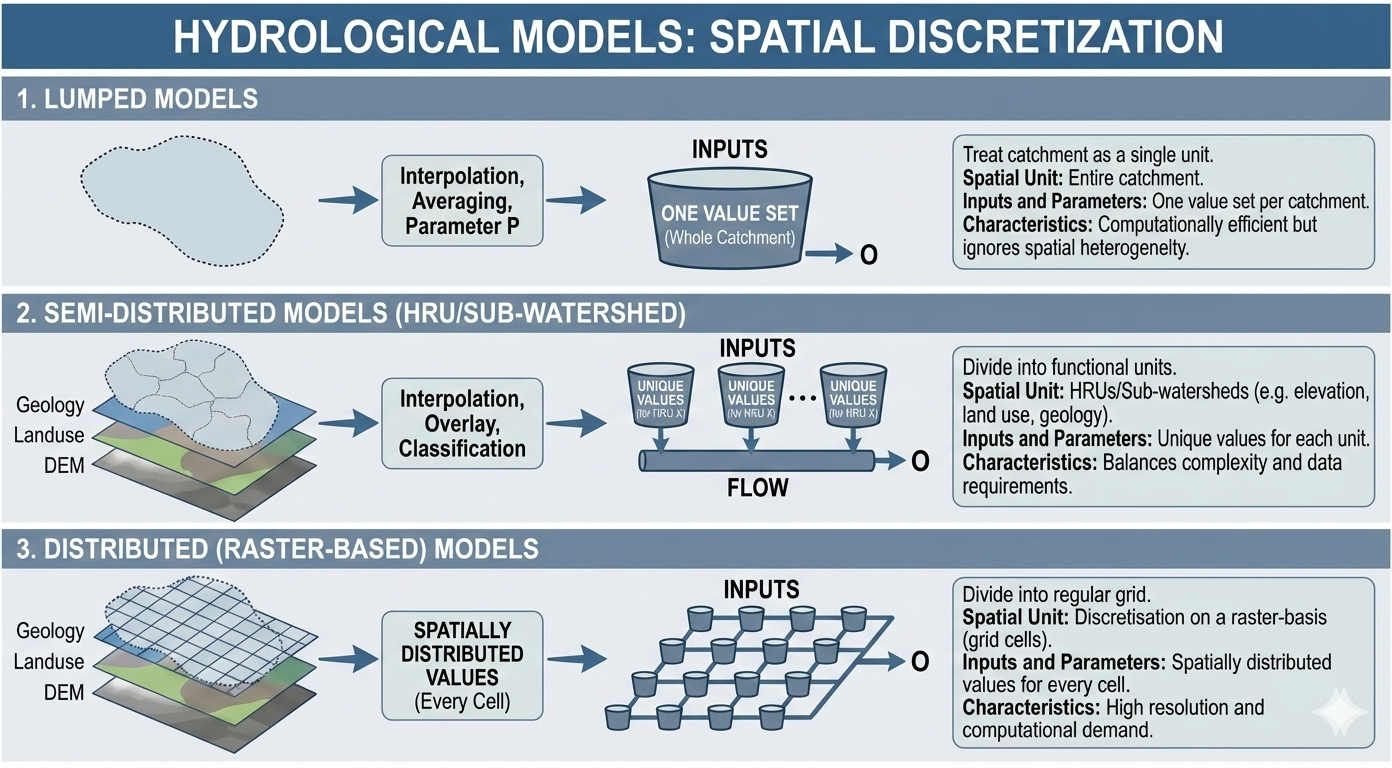
COSERO offers the flexibility to run in a fully distributed (gridded) mode, but also in a semi-distributed or lumped approach. It uses a hierarchical system to represent the river catchment, dividing it into Subbasins and Zones.
The catchment is first divided into several subbasins. For the outlet of each subbasin, the model computes a simulated discharge (\(Q_{sim}\)).
To account for physical heterogeneity within a subbasin, a further subdivision into Model Zones (NZ/IZ) is performed. IZ reflects zones within a subbasin and NZ the zone ID within the total model. These zones act as the fundamental calculation units and can be defined using different concepts:
Regardless of whether they are HRUs or grid cells, the zones (NZ) are the basic spatial modelling units. Each zone:
Within the subbasin, the outflow of all zones is aggregated and, together with inflow from upstream subbasins, is routed to the basin outlet to form the subbasin runoff.
Model parameters are spatially distributed across the subbasin and have the dimensions defined by the hierarchy (Subbasin NB, Zone within a subbasin IZ). Some parameters also include a temporal dimension (e.g., maximum interceptions storage, which varies on a monthly basis).
| Dimension | Description |
|---|---|
| NB | Index of Subbasin |
| IZ | Index of Zone in subbasin |
| NZ | Index of Zone in total model |
| NM | Month index (1-12) |
| NC | Vegetation / land cover class index |
| IKL | Total number of snow classes per zone |
| IZONE | Total number of zones per subbasin |
| NBASIN | Total number of subbasins |
| NCLASS | Total number of vegetation / land cover classes |
Establishing a hydrological model follows a systematic workflow involving four main stages (Figure 4).
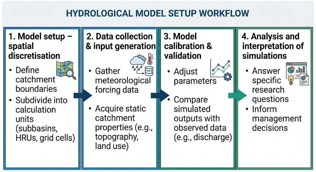
To execute these steps, the model generally requires three categories of data:
For catchments in Austria, high-quality datasets are available for all three categories.

For meteorological input data in Austria, the an important source is the GeoSphere Austria Data Hub. This initiative is a exemplary and commendable effort: by making high-quality weather, climate, environmental, and geophysical datasets freely and openly accessible to researchers, public institutions, and commercial users alike, GeoSphere Austria sets a benchmark for open science and data-driven innovation.
For modelling purposes, we typically distinguish between daily and hourly meteorological products.
The Spatially Resolved Temperature and Precipitation Climatology for Austria is the standard dataset for daily modeling.
| Attribute | Details |
|---|---|
| Source | GeoSphere Data Hub |
| DOI | 10.60669/m6w8-s545 |
| Resolution | 1 km × 1 km; Daily |
| Parameters | Precipitation (RR), Min/Max Temperature (TN, TX) |
Note — Day definition and temporal alignment: SPARTACUS daily values do not follow the standard calendar day (00:00–00:00 CET). Precipitation (RR) is accumulated over 07:00–07:00 CET, while minimum and maximum temperature (TN, TX) are defined as the extremes of the 19:00–19:00 CET interval. Observed discharge from eHYD/HZB, by contrast, uses the standard 00:00–00:00 day. When processing SPARTACUS data with
write_spartacus_precip()andwrite_spartacus_temp()in the CoseRo package, a temporal shift is applied by default (time_shift = TRUE) to harmonise all inputs to the 00:00–00:00 convention before writing the COSERO input files. This correction should always be applied when combining SPARTACUS with eHYD discharge records.Mean temperature (\(TM\)) can be calculated as \(TM = \frac{TN + TX}{2}\), though the CoseRo package provides more sophisticated methods (e.g., the Dall’Amico approach) that account for the temperature distribution within the day.
The Integrated Nowcasting through Comprehensive Analysis (INCA) system is used for high-resolution, sub-daily modeling (e.g., flood forecasting). It combines station observations, remote sensing (radar), and numerical weather prediction models.
| Attribute | Details |
|---|---|
| Source | GeoSphere Data Hub |
| DOI | 10.60669/6akt-5p05 |
| Resolution | 1 km × 1 km; 15-Minutes (Precipitation) and Hourly |
| Projection | MGI / Austria Lambert (EPSG: 31287) |
| Parameters | Temperature, Precipitation, Wind, Global Radiation, Humidity |
For applications requiring raw station data (which must be interpolated), observations can be accessed via:
Note — Sub-daily data: The publicly available eHYD datasets are limited to daily resolution. For applications requiring sub-daily (e.g., hourly) precipitation or temperature records — such as flood forecasting or urban hydrology — data must be requested directly via email.
The eHAO offers thematic GIS layers representing the nation’s hydrological characteristics, such as soil types, land use, and water balance components.
The eHYD platform is the primary source for hydrographic observation data in Austria.
Note — Sub-daily data: The eHYD platform provides discharge data at daily resolution. For applications requiring sub-daily (e.g., hourly or 15-minute) discharge records — such as flood forecasting or event-based modelling — data must be requested directly via email.
For applications outside of Austria or for large-scale studies, many global datasets for setting up hydrological models exist. Here is an incomplete list:
| Category | Dataset | Description | Link |
|---|---|---|---|
| Discharge & Catchment | GRDC | Global Runoff Data Centre. River discharge data for over 10,000 stations worldwide. | bafg.de |
| CAMELS | Catchment Attributes and Meteorology for Large-sample Studies. Standardized datasets (meteo, discharge, soil, land use) for specific regions (USA, GB, AUS, BR, CL, etc.). | NCAR | |
| LamaH-CE | Large-Sample Data for Hydrology for Central Europe. A CAMELS-like dataset covering the Danube and Rhine basins (over 850 catchments). | Zenodo | |
| Topography (DEM) | HydroSHEDS | Hydrological products based on SRTM (3 arc-sec), offering conditioned river networks, watershed boundaries, and drainage directions. | hydrosheds.org |
| MERIT Hydro | Multi-Error-Removed Improved-Terrain. A globally corrected DEM (~90m) specifically processed for hydrology (removal of tree canopy/noise). | U-Tokyo | |
| COP30 / TanDEM-X | Copernicus GLO-30 and TanDEM-X. High-precision global DEMs at ~30m (1 arc-sec) and ~12m resolution respectively. | ESA | |
| Meteorology (Reanalysis) | ERA5 | Global atmospheric reanalysis from ECMWF. Hourly estimates of atmospheric variables on a ~30km grid (1950–present). | ECMWF |
| ERA5-Land | A downscaled version of ERA5 specifically for the land component. Provides hourly data at 9km resolution, better suited for catchment modeling. | CDS | |
| Precipitation (Satellite/Merged) | MSWEP | Multi-Source Weighted-Ensemble Precipitation. Merges gauge, satellite, and reanalysis data for high-quality global precip estimates (3-hourly, 0.1°). | GloH2O |
| CHIRPS | Climate Hazards Group InfraRed Precipitation with Station data. Rainfall data (daily, 0.05°) specifically designed for trend analysis and drought monitoring (50°S-50°N). | CHG | |
| GPM IMERG | Integrated Multi-satellitE Retrievals for GPM. NASA’s high-resolution (0.1°, 30-min) satellite precipitation product. | NASA | |
| Soil & Land Cover | HWSD | Harmonized World Soil Database. A global soil raster database providing parameters (texture, bulk density, carbon) for modeling. | FAO |
| SoilGrids | Global soil information system providing prediction of soil properties at 250m resolution using machine learning. | ISRIC | |
| ESA WorldCover | High-resolution (10m) global land cover map based on Sentinel-1 and Sentinel-2 data (versions 2020/2021). | ESA |
To bridge the gap between theoretical hydrological concepts and practical application, we utilize a specific software stack. The workflow integrates QGIS for spatial data processing, R for data preparation and analysis, and the COSERO hydrological model engine.
The core COSERO.exe model is a Windows-only executable. Therefore, a Windows operating system is required to run simulations. Users on macOS or Linux will need a virtual machine or emulation layer to execute the model core.
If you need a refresher on R fundamentals — data types, vectors, data frames, dplyr, or ggplot — work through the R & RStudio Introduction supplementary resource before continuing.
![]() CoseRo (v0.9.0) provides a complete R interface for the COSERO hydrological model, covering the full modelling lifecycle — from downloading and preprocessing input data, through running simulations and reading outputs, to sensitivity analysis, parameter calibration, and interactive result exploration.
CoseRo (v0.9.0) provides a complete R interface for the COSERO hydrological model, covering the full modelling lifecycle — from downloading and preprocessing input data, through running simulations and reading outputs, to sensitivity analysis, parameter calibration, and interactive result exploration.
The package is hosted on GitHub. The recommended approach uses the remotes package; all core dependencies are installed automatically.
install.packages("remotes")
remotes::install_github("Herrnegger/CoseRo")Optional packages required for spatial preprocessing (SPARTACUS/WINFORE) and data download must be installed separately:
# For SPARTACUS/WINFORE spatial preprocessing
install.packages(c("terra", "sf", "exactextractr", "future", "furrr"))

# For GeoSphere Austria data download
install.packages("httr")

# For SCE-UA optimisation
install.packages("rtop")The fastest way to get started is to create the bundled Wildalpen example project and explore it in the Shiny app:
library(CoseRo)

# Create a ready-to-run example project (Salza/Wildalpen catchment)
setup_cosero_project_example("C:/COSERO/Wildalpen")  # adjust path

# Launch the interactive app with data pre-loaded
launch_cosero_app("C:/COSERO/Wildalpen")The table below summarises all main functions grouped by task. Functions used in this course are covered in more detail in the relevant module.
| Group | Function | Description |
|---|---|---|
| Model Execution | run_cosero() |
Execute a COSERO simulation with custom settings and warm/cold start |
launch_cosero_app() |
Launch the interactive Shiny app | |
| Project Setup | setup_cosero_project_example() |
Create a ready-to-run example project (Wildalpen catchment) |
setup_cosero_project() |
Create an empty COSERO project directory structure | |
| Output Reading | read_cosero_output() |
Read all COSERO output files (auto-detects OUTPUTTYPE 1–3) |
read_cosero_parameters() |
Read the parameter file (para.txt) |
|
get_subbasin_data() |
Extract discharge data for a specific subbasin | |
| Single Run Metrics | extract_run_metrics() |
Extract performance metrics from single-run statistics output |
calculate_run_metrics() |
Calculate metrics directly from QSIM vs QOBS | |
| Sensitivity Analysis | load_parameter_bounds() |
Load parameter bounds from the bundled CSV |
generate_sobol_samples() |
Generate Sobol quasi-random parameter sets | |
run_cosero_ensemble() |
Run ensemble simulations (sequential) | |
run_cosero_ensemble_parallel() |
Run ensemble simulations (parallel, recommended) | |
extract_ensemble_metrics() |
Extract metrics from ensemble statistics output | |
calculate_ensemble_metrics() |
Calculate metrics from ensemble QSIM/QOBS | |
calculate_sobol_indices() |
Calculate first-order and total-order Sobol indices | |
plot_sobol() |
Visualise Sobol sensitivity indices | |
plot_dotty() |
Parameter–output scatter plots (dotty plots) | |
plot_ensemble_uncertainty() |
Ensemble discharge uncertainty with observed overlay | |
plot_metric_distribution() |
Distribution of performance metrics across ensemble | |
extract_behavioral_runs() |
Filter behavioural runs by NSE/KGE/pBias criteria | |
| Parameter Optimisation | optimize_cosero_dds() |
DDS algorithm — fast, recommended for 3–10 parameters |
optimize_cosero_sce() |
SCE-UA algorithm — robust global optimisation | |
create_optimization_bounds() |
Define parameter bounds for optimisation | |
plot_cosero_optimization() |
Plot optimisation convergence history | |
export_cosero_optimization() |
Export optimisation results and report | |
| Input Preprocessing | download_geosphere_data() |
Download SPARTACUS/WINFORE NetCDF files from GeoSphere Austria |
write_spartacus_precip() |
Convert SPARTACUS precipitation to COSERO input format | |
write_spartacus_temp() |
Convert SPARTACUS Tmin/Tmax to COSERO Tmean input format | |
write_winfore_et0() |
Convert WINFORE ET₀ to COSERO input format | |
write_ehyd_qobs() |
Convert eHYD discharge CSV files to COSERO QOBS format |
Before the next session, please ensure the following are in place:
After completing this module you should understand the following concepts and be able to explain them in your own words. These points may also serve as a guide for your presentation.
defaults.txt, parameter file, meteorological inputs, QOBS file). Identify which data sources are used in Austria and which global alternatives exist.Document created: 2026-05-22