Mathew Herrnegger · mathew.herrnegger@boku.ac.at
Institute of Hydrology and Water Management (HyWa) BOKU University Vienna, Austria
LAWI301236 · Distributed Hydrological Modeling with COSERO
![]()
Course Overview
![]()
This seminar provides hands-on experience with distributed hydrological modeling using COSERO, a flexible rainfall-runoff model. Working in small groups, you will set up, parameterize, and run COSERO for real catchments, applying the full workflow from spatial data processing to model evaluation.
Computational Thinking in Hydrological Modelling
The core of this course is not simply learning to program in R or applying a specific software — it is developing or strengthening Computational Thinking. This means
- decomposing problems,
- identifying patterns,
- abstracting complex realities, and
- designing step-by-step algorithms.
In applied hydrology it also means mastering the full modelling workflow.
Simulating the hydrological cycle requires different tools: GIS software like QGIS for spatial data processing, spreadsheets for quick analysis, scripting languages like R to prepare inputs and analyse outputs, and numerical models — often written in Fortran or C++ — to run the actual simulations. Computational thinking is also what allows you to decide which tool is right for each step and how to chain them together coherently, moving from raw data to a reliable, reproducible result.
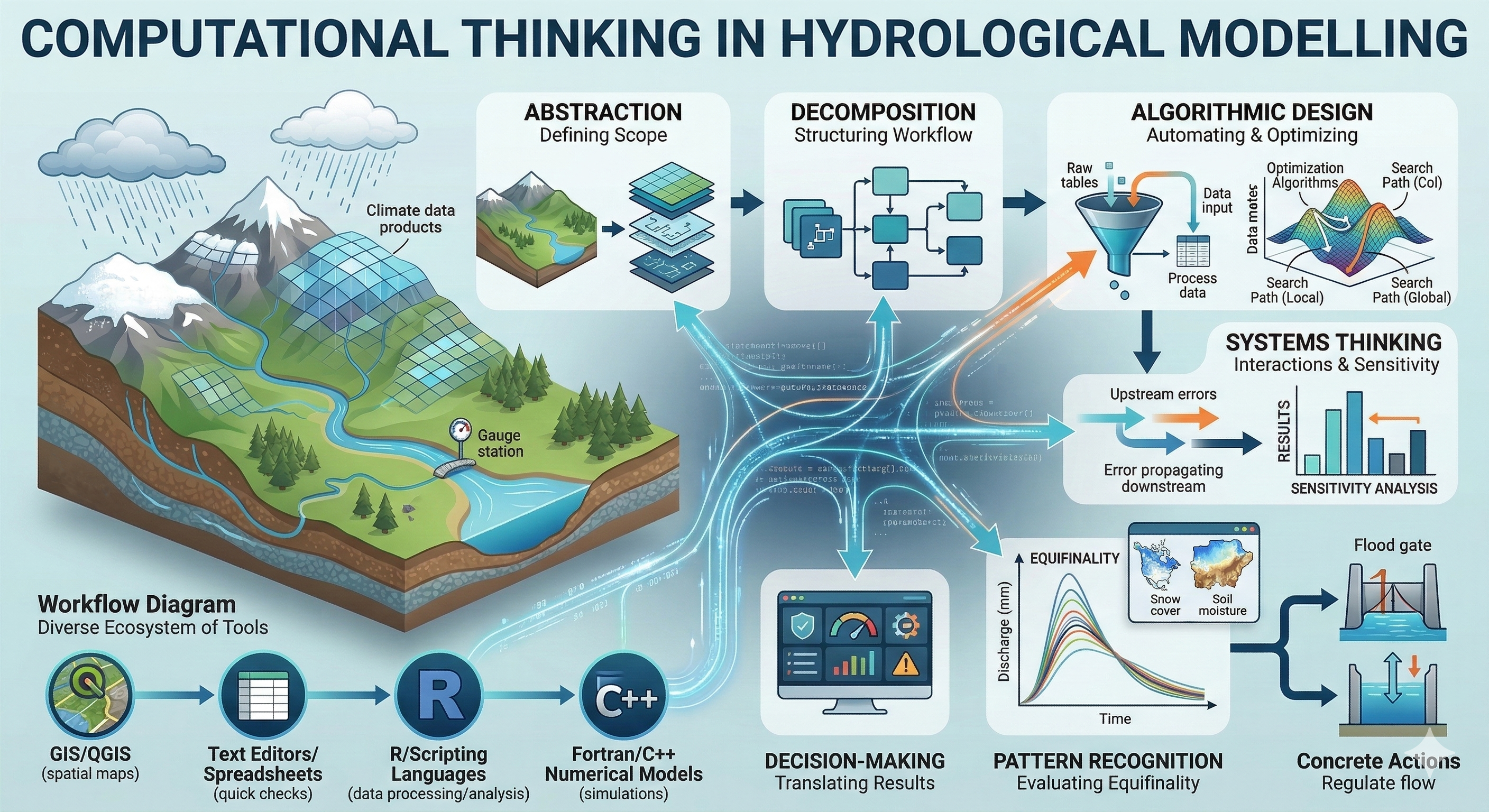
Getting from physical understanding to prediction — and ultimately to decision-making — requires breaking the challenge into distinct, manageable layers.
Abstraction comes first: before opening any software, you define the scope of the problem, determining which outputs are needed and which inputs are strictly necessary. Recognising, for example, that a 1-metre elevation model is overkill for a 10-kilometre climate grid is itself a non-trivial modelling decision.
From there, decomposition structures the entire workflow — separating spatial pre-processing in QGIS from time-series formatting in R and the core simulation in Fortran or C++, so that each step has a clear owner and a clear output.
Once the workflow is structured, algorithmic thinking replaces manual, error-prone data handling with explicit, repeatable scripts. This applies equally to calibration: rather than adjusting parameters by hand, we select and apply systematic optimisation algorithms — whether local gradient-based methods or global evolutionary strategies — to search the parameter space efficiently. But no algorithm operates in isolation.
Systems thinking reminds us that a catchment model is a strong simplification of an interconnected system, where humans influence flow, e.g. due to hydropower, or upstream errors propagate downstream, and where changing one model parameter can alter the sensitivity of another. Sensitivity analysis is therefore handy; it is how we find out which parameters actually control the output.
Even after a calibration, pattern recognition demands critical scrutiny of the results. Good statistical metrics are necessary but not sufficient — equifinality means that multiple different parameter sets can produce equally plausible hydrographs. We must look beyond the numbers and check whether the model reproduces internal states such as snow cover or soil moisture for the right physical reasons or if the water balance is closed correctly.
Only then can the final step, decision-making, be carried out responsibly: translating simulation results and their associated uncertainties into concrete, actionable insights for flood forecasting, reservoir management, or climate impact assessments.
None of this is straightforward. Each layer requires turning a vague physical understanding into a sequence of concrete, unambiguous operations. The R code you write in this course is not the ultimate goal; it is the medium that forces you to be absolutely explicit about every assumption, every parameter choice, and every analytical decision.
Modules
The course is structured into four modules that follow the complete modelling workflow — from understanding the model and preparing the data, through first exploratory runs and sensitivity analysis, to systematic calibration and in-depth output interpretation.
Module 1: Introduction & Model Structure
An introduction to distributed hydrological modelling and the COSERO model.
- Why rainfall-runoff transformation is non-linear and why we need models
- COSERO history, development, and applications in Austria and the World
- Model process representation: snow accumulation & melt, soil water & interception, three-component discharge routing
- Spatial discretisation: lumped catchments, semi-distributed zones, and HRUs
- Data sources: SPARTACUS, WINFORE, eHAO, eHYD, and global alternatives
- Software environment: R, QGIS, and the CoseRo package
Module 2: Spatial Structure & Meteorological Inputs
The practical foundation for building a COSERO model from scratch.
- Subbasin delineation and catchment setup in QGIS
- Generating COSERO model zones with IDs and routing topology
- Deriving initial parameters from Austria-wide raster datasets
- Processing SPARTACUS gridded precipitation and temperature into COSERO input files
- Processing WINFORE potential evapotranspiration
- Preparing observed discharge records from eHYD
Module 3: Parameter Estimation & Sensitivity
The first hands-on encounter with a running model.
- Executing an initial simulation with user defined parameters
- Interactive result exploration with the CoseRo Shiny app
- Performance metrics: NSE, KGE, and volume bias (BETA)
- Programmatic parameter modification and scenario comparison
- Global Sobol sensitivity analysis to identify the parameters that actually control model behaviour
Module 4: Calibration, Validation & Output Analysis
Systematic model optimisation and thorough result interpretation.
- DDS automatic calibration using Sobol-informed parameter bounds
- Split-sample calibration and validation with performance assessment
- Hydrograph analysis: full period, event zooms, flow duration curves, and residuals
- Seasonal dynamics: monthly discharge regime, NSE, and water balance
- Water balance components and runoff generation (surface, interflow, baseflow)
- Spatial visualisation of calibrated parameters across zones
Case Study: Salza River (Wildalpen)
Throughout this course, we use the Salza catchment in the Hochschwab region as demonstration example for model setup and calibration. The map below shows the study area with sub-catchment boundaries, river network, and gauging stations.
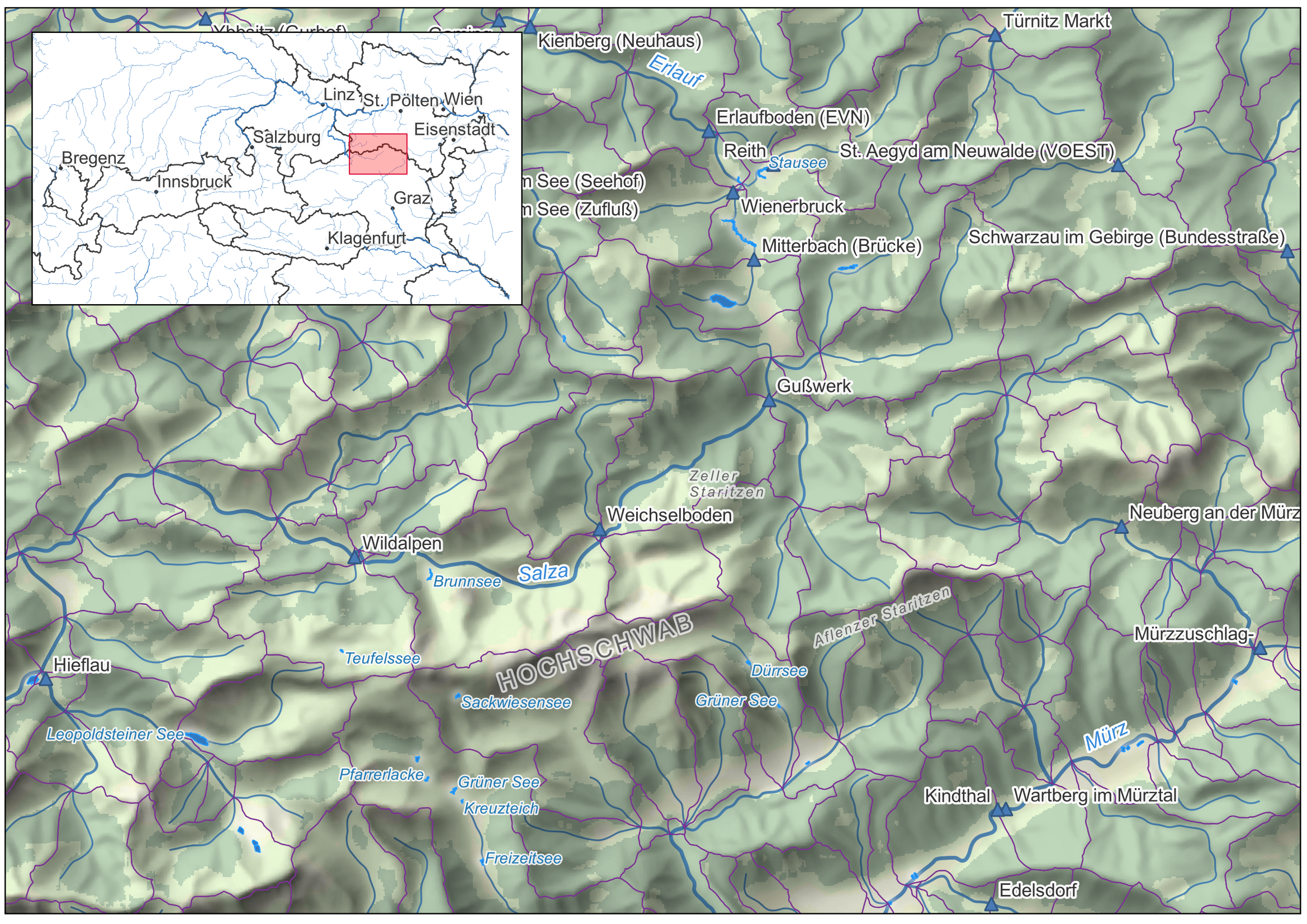
For your group project, you will select a different catchment. The Salza example demonstrates the complete workflow you will apply to your own study area.
Getting Started
Group Formation
As we move into the practical application phase in Module 2, you will work in small teams.
- Form groups: 2-3 students per group.
- Assignment: Each group will be responsible for setting up, calibrating, and analyzing a specific Austrian catchment (different from the Salza demo case).
- Workflow: Coordinate within your group to ensure consistent file management and data processing.
- Group presentation: At the end of the course, you will present your data, modelling experiences and challenges. Have this in mind while working and modelling.
Catchment Selection
In the next session, you will select a catchment from the Hydrological Atlas. To ensure a successful modeling exercise, your selection should meet the following criteria:
- Observation Data: Reliable discharge records must be available via eHYD.
- Record Length: A sufficient data period (≥10 years) is recommended to allow for split-sample calibration and validation.
- Scale: Manageable catchment size suitable for the course with a total size of < 1000 km² and which also includes discharge data of sub-catchments.
- Characteristics: Distinct hydrological features (e.g., purely alpine, lowland, or mixed regimes) are encouraged to observe different process dominances.
Prerequisites
Required:
- LAWI301241 Exercises in Hydrological Processes and Water Resources Management
- Proficient R/RStudio programming — if you need a refresher, see the R & RStudio Introduction
- Basic QGIS skills
Beneficial:
- LAWI301244 Application of GIS in Hydrology and Water Management
Resources
- R & RStudio Introduction
- COSERO Handbook
- ÖWAV-Regelblatt 220: Rainfall-Runoff Modelling — Austrian technical guideline (2019, 368 pages) published by the ÖWAV (Austrian Water and Waste Management Association)
- Data Hub of GeoSphere Austria
- eHYD - Hydrographic Data
- Hydrological Atlas of Austria
Learning Outcomes
What You Should Know
By the end of this course you should be able to work confidently with a spatially distributed hydrological model from raw data to calibrated output. The following four areas summarise the core competencies, each built up progressively across the four modules.
Model structure and spatial setup (Modules 1 & 2) Explain the COSERO state-space concept and how precipitation and temperature are transformed into discharge through snow, soil, runoff generation, and baseflow processes. Set up a distributed model from scratch: delineate subbasins in QGIS, generate initial parameters from landscape raster maps for COSERO zones, process SPARTACUS and WINFORE meteorological inputs, and assemble all required input files. Understand why zone-level parameter variability can rarely be measured in reality.
Parameter sensitivity and behavioural filtering (Module 3) Apply variance-based Sobol sensitivity analysis to identify which parameters control model performance and which interact. Interpret dotty plots and distinguish between sensitivity and identifiability. Apply multi-objective behavioural filtering to isolate acceptable parameter combinations, quantify parameter uncertainty, and save the best-performing parameter set as a COSERO input file ready for Module 4.
Calibration and validation (Module 4) Use the DDS algorithm to automatically calibrate selected parameters within physically motivated bounds. Conduct a split-sample validation and critically evaluate whether calibration performance is sustained over an independent period. Understand what a drop in validation performance implies about model structure, data quality, or equifinality.
Model evaluation and physical plausibility (Modules 3 & 4) Go beyond aggregate metrics: inspect hydrographs at the event scale, decompose performance by season, verify water balance closure, and map spatial patterns in calibrated parameters. Articulate the limitations of your model, identify which processes are least well represented, and propose physically motivated directions for improvement — keeping in mind that a high NSE does not guarantee a correct model.